Bridging the Gap between Theory and Simulation in the Bottleneck Model
Lucas Javaudin, André de Palma
THEMA, CY Cergy Paris Université
ITEA 2024
Outline
- Transport Simulators: Gap to the Theory
- Methodology
- Results
- Large-Scale Simulations
- Conclusion
The Bottleneck Model in Simulators: Inspiration
- Bottleneck model (Vickrey, 1969; Arnott, de Palma, Lindsey, 1990s): single-road, alpha-beta-gamma generalized cost
- Transport simulators: tools to evaluate transport policies in large-scale scenarios
- MATSim and METROPOLIS use bottleneck congestion: flows are limited by road capacity
- SimMobility and METROPOLIS use alpha-beta-gamma generalized cost with departure-time choice
- Apart from these inspirations, transport simulators are complex black boxes
- To what extent are their results in line with theory?
Analytical Model vs Simulation
| Analytical model | Simulation | |
|---|---|---|
| Population | Continuum of individuals | Discrete agents |
| Choice model | Deterministic | Random-utility model |
| Behavioral representation | Continuous, implicitly-defined | Piecewise-linear, numerical approximation |


Attempts at Simulating the Bottleneck Model
-
Otsubo and Rapoport (2008)
- Discrete agents and mixed-strategy equilibrium
- "We report significant discrepancies in travel costs and distributions of departure time between the two solutions that slowly decrease as the number of commuters increases."
- Methodology limited to very simple networks
-
Guo, Yang, Huang (2018)
- Continuum of individuals, deterministic choice model
- "We theoretically prove that, in the simplest standard bottleneck model [...], a dynamic user equilibrium (DUE) cannot be reached through a day-to-day evolution process of travelers’ departure rate"
Contributions
- We propose a methodology able to replicate the analytical results of the bottleneck model
- Framework: discrete agents, random-utility model
-
Solution:
- Continuous departure-time choice (de Palma, Ben-Akiva, Lefèvre and Litinas, 1983)
- Continuous-time model
- Optimal at each iteration
- This methodology is then extended into a large-scale transport simulator: METROPOLIS2
The Bottleneck Model
-
Single-road network:
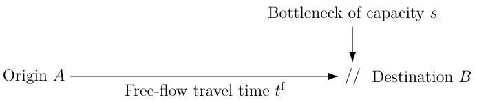
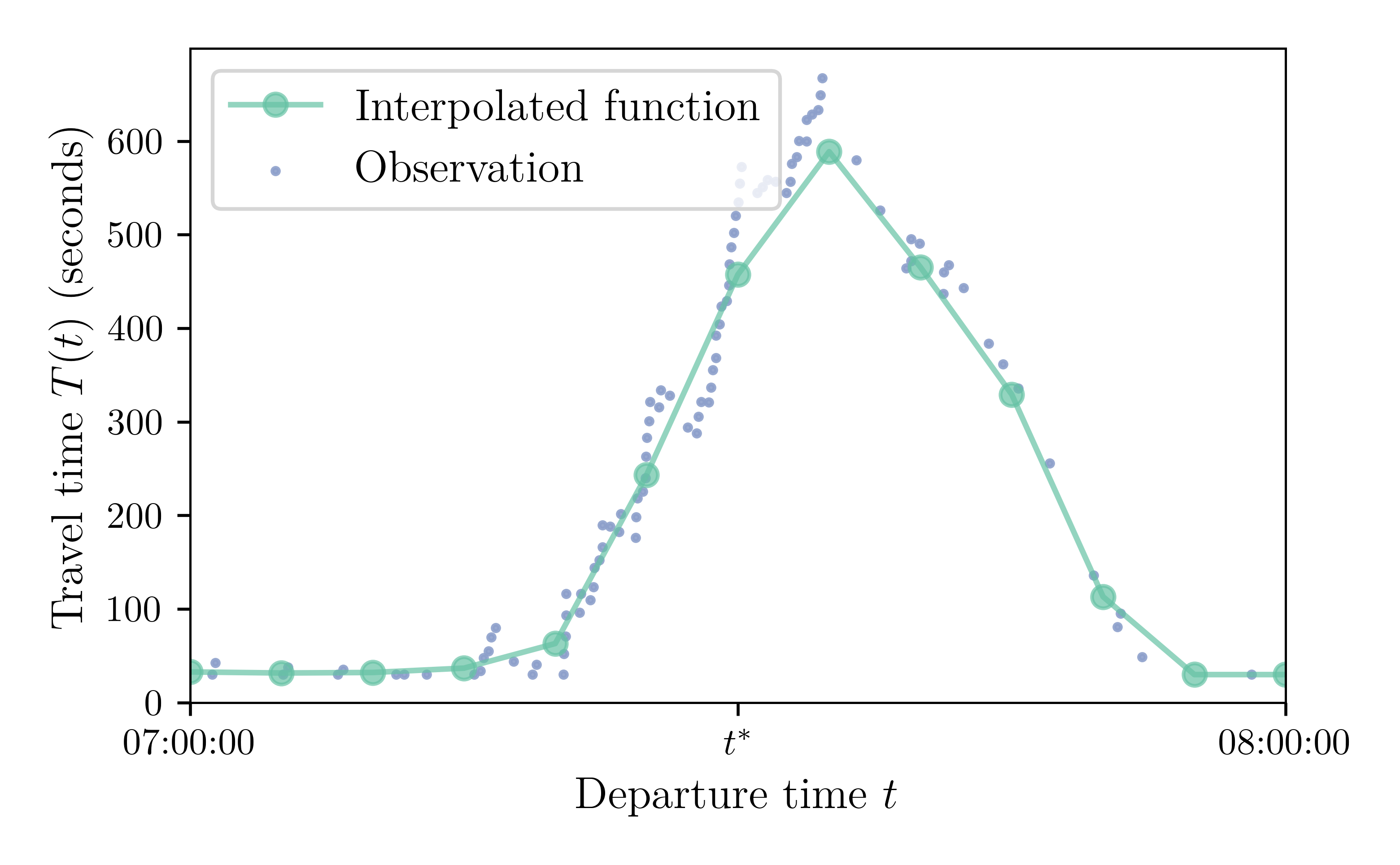
- Travel time from $A$ to $B$ is \[ t^f + \frac{Q(t + t^f)}{s} \] with $Q$ the length of the bottleneck queue at time $t$.
- $N$ discrete agents are traveling from Origin $A$ to Destination $B$
- Utility ($\approx$ generalized cost) is given by \[ V(t) = -\alpha \cdot T(t) - \beta \cdot [t^* - t - T(t)]_+ - \gamma \cdot [t + T(t) - t^*]_+ \]
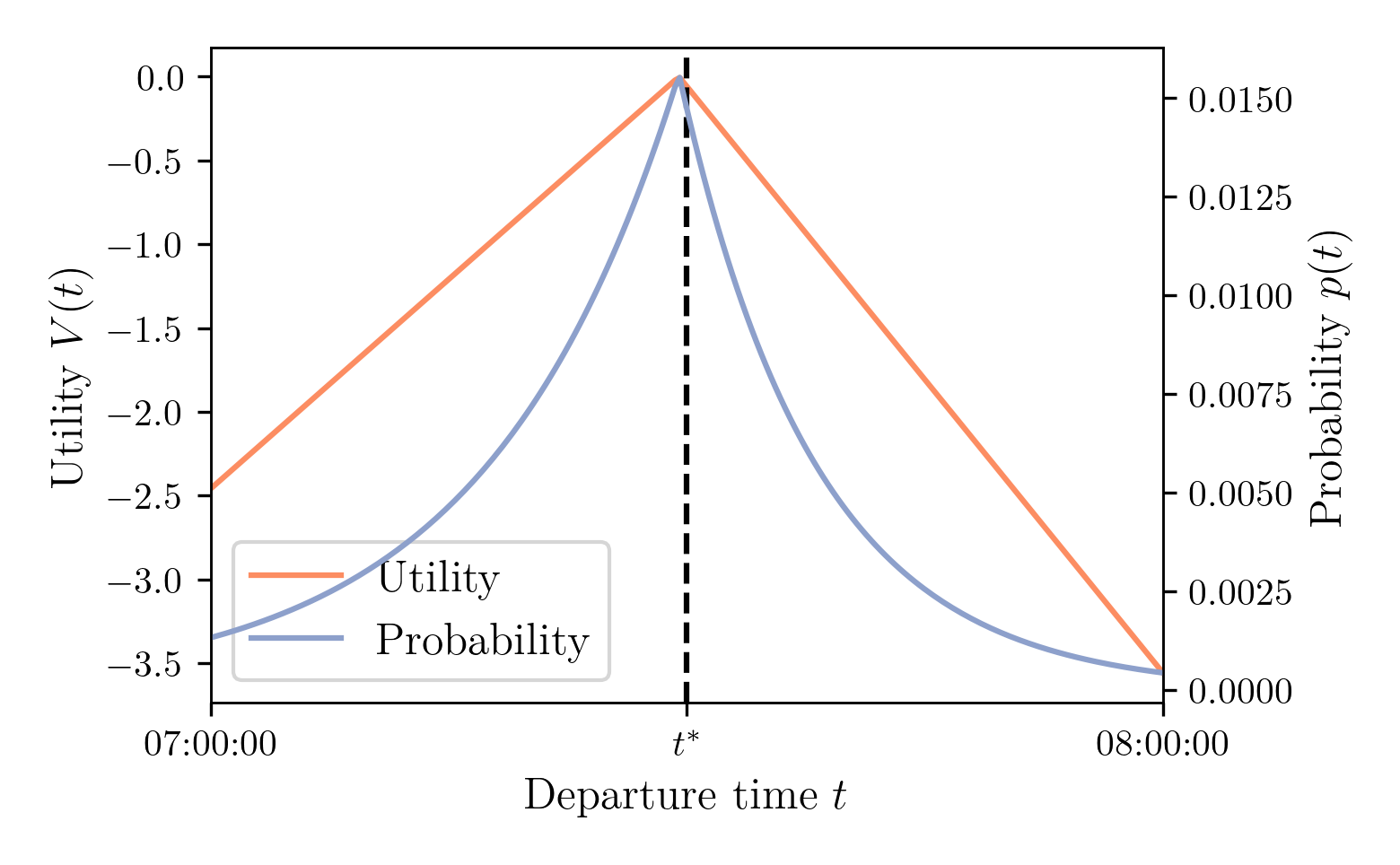
The Bottleneck Model: Departure-Time Choice
- Agents choose the departure time maximizing deterministic utility (Arnott, de Palma and Lindsey, 1990): \[ t^d = \arg \max V(t) \]
- Agents choose departure time $t$ with probability (Continuous Logit, de Palma, Ben-Akiva, Lefèvre and Litinas, 1983): \[ p(t) = \frac{e^{V(t) / \mu}}{\int_{t^0}^{t^1} e^{V(\tau)/\mu} d \tau} \]
- Fixed-point problem: $p(t) \leftrightarrow V(t)$
- Alternative interpretation: mixed strategy

Iterative Process
Initial conditions
|
||||
| ↓ Demand model ↑ |
⟶ |
|
⟶ | Supply model ↓ |
|
⟵ | Learning model ↓ |
⟵ |
|
| Stopping rule |
Demand Model
-
Compute utility function from the expected travel-time function $\hat{T}$:
\[ V(t) = -\alpha \cdot \hat{T}(t) - \beta \cdot [t^* - t - \hat{T}(t)]_+ - \gamma \cdot [t + \hat{T}(t) - t^*]_+ \]
-
Compute the departure-time probabilities from the Continuous Logit formula:
\[ p(t) = \frac{e^{V(t) / \mu}}{\int_{t^0}^{t^1} e^{V(\tau)/\mu} d \tau} \]
- Draw departure times using inverse transform sampling

Supply Model
- An event-based model is used to simulate the trips of all the agents, from origin to destination
- To simulate a bottleneck of capacity $s$ vehicles per time unit, the road outflow is blocked for $1 / s$ time units after each vehicle is crossing
- Example: bottleneck capacity 1800 vehicles / hour ↔ closing time 2 seconds
- FIFO: The cars exit the bottleneck in the same order that they entered it
- Continuous time: It can work with very small or very large capacities
Learning Model
- The travel-time function expected for the next iteration, $\hat{T}_{\kappa+1}$, depends on the simulated travel-time function, $T_\kappa$, and the expected travel-time function, $\hat{T}_\kappa$, of the current iteration.
-
Exponential smoothing method:
\[ \hat{T}_{\kappa + 1} = \lambda T_\kappa + (1 - \lambda) \hat{T}_{\kappa} \]with $\lambda \in [0, 1]$, the smoothing factor.
- An equilibrium is reached when $\hat{T}_{\kappa} = T_{\kappa}$
$\hat{T}_{\kappa}$
$T_{\kappa}$
$\hat{T}_{\kappa + 1}$
Simulations
- $N = 100,000$ agents
- $\alpha = 10\$ / h$, $\beta = \gamma = 5\$ / h$
- $t^*$ = 7:30 a.m.
- Free-flow travel time $t^f$ = 30 seconds
- Bottleneck capacity $s = 150,000$ cars / h
- Smoothing factor $\lambda = 0.5$
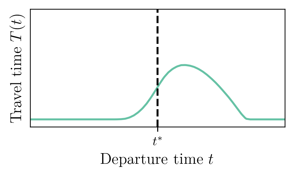
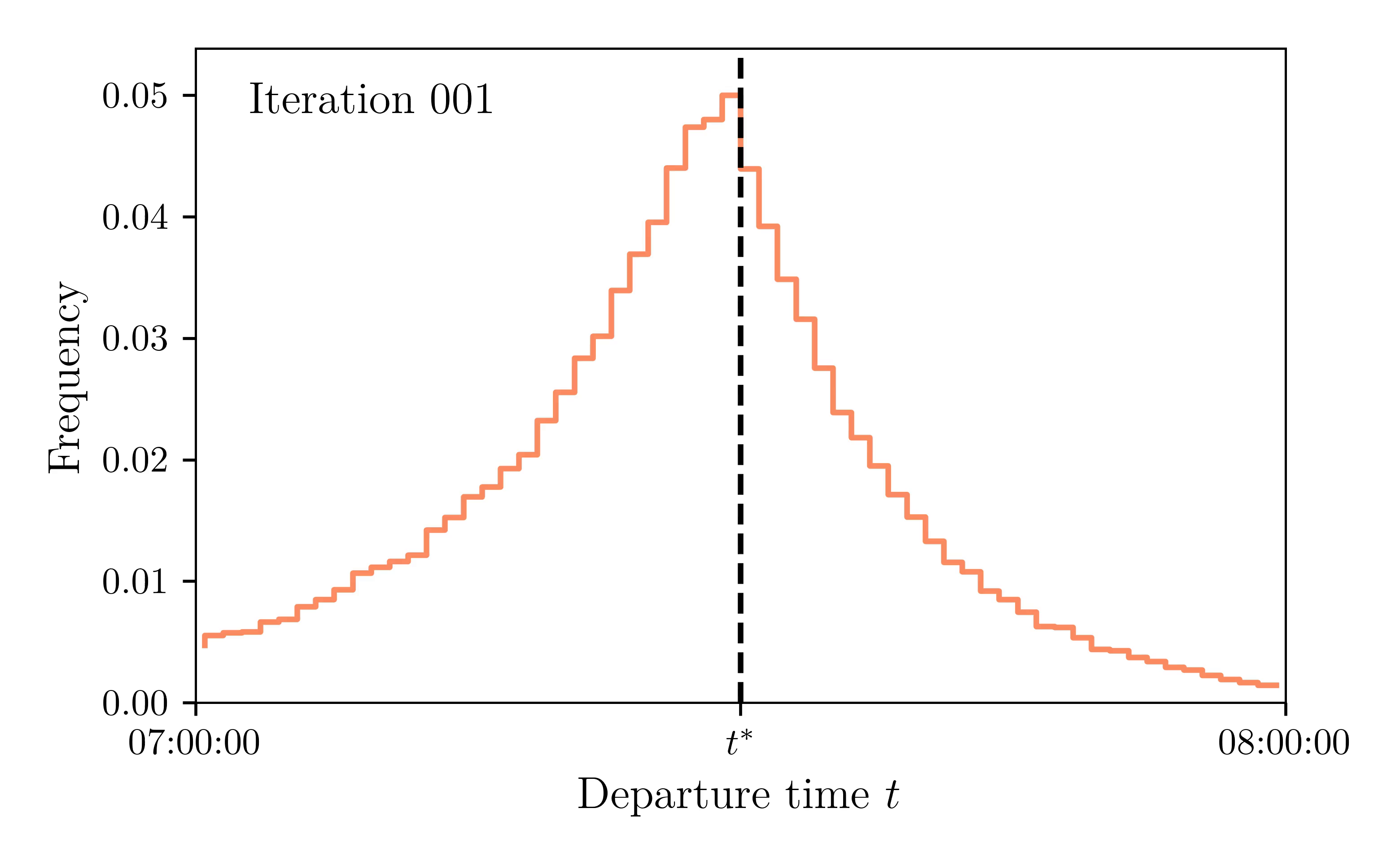
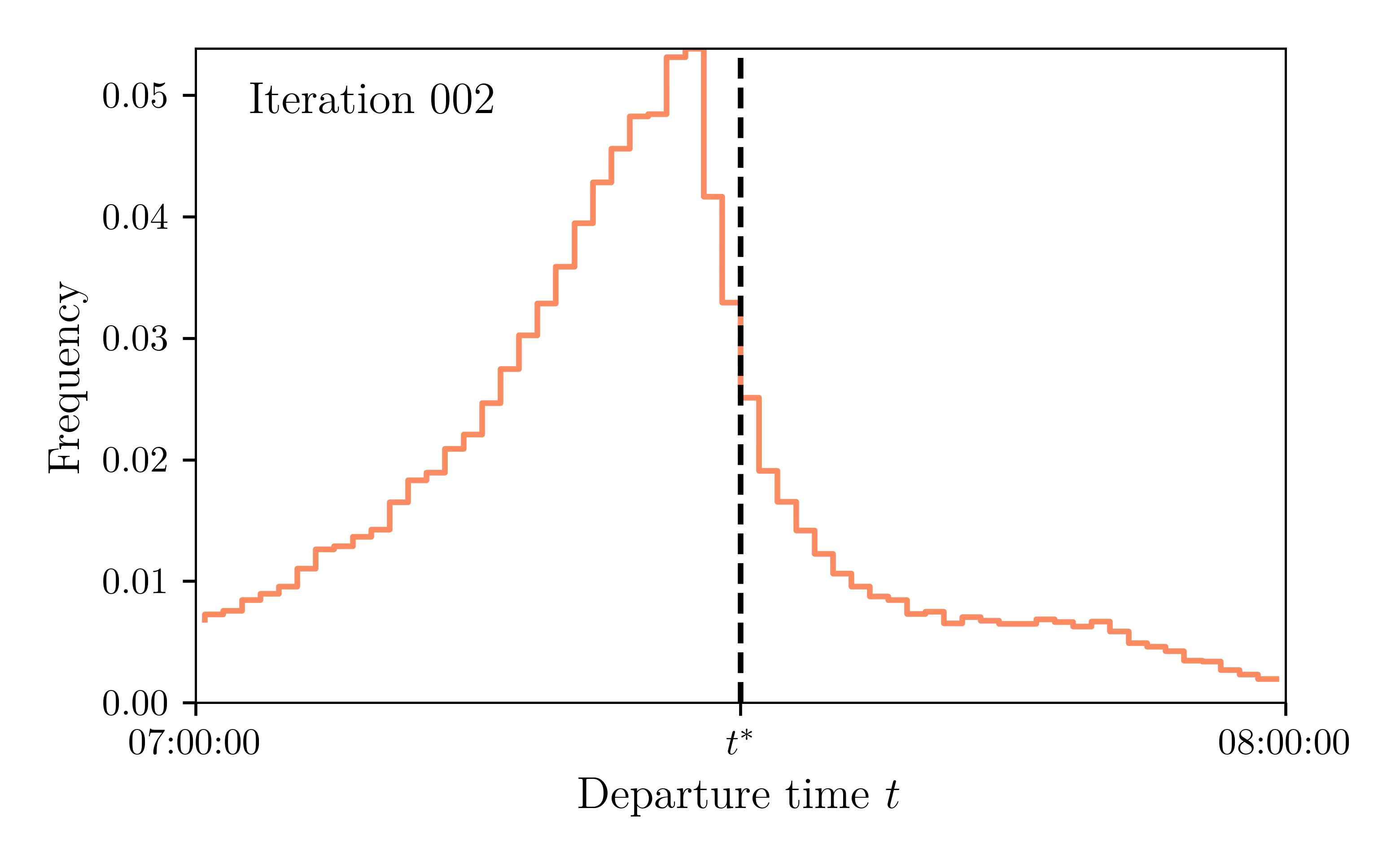
Departure rate: Iteration 1 & 2
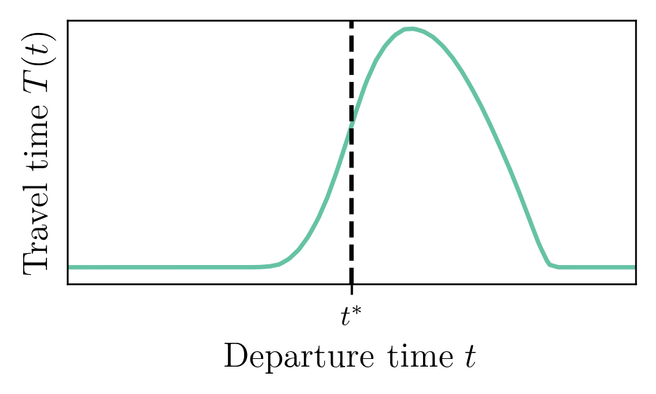
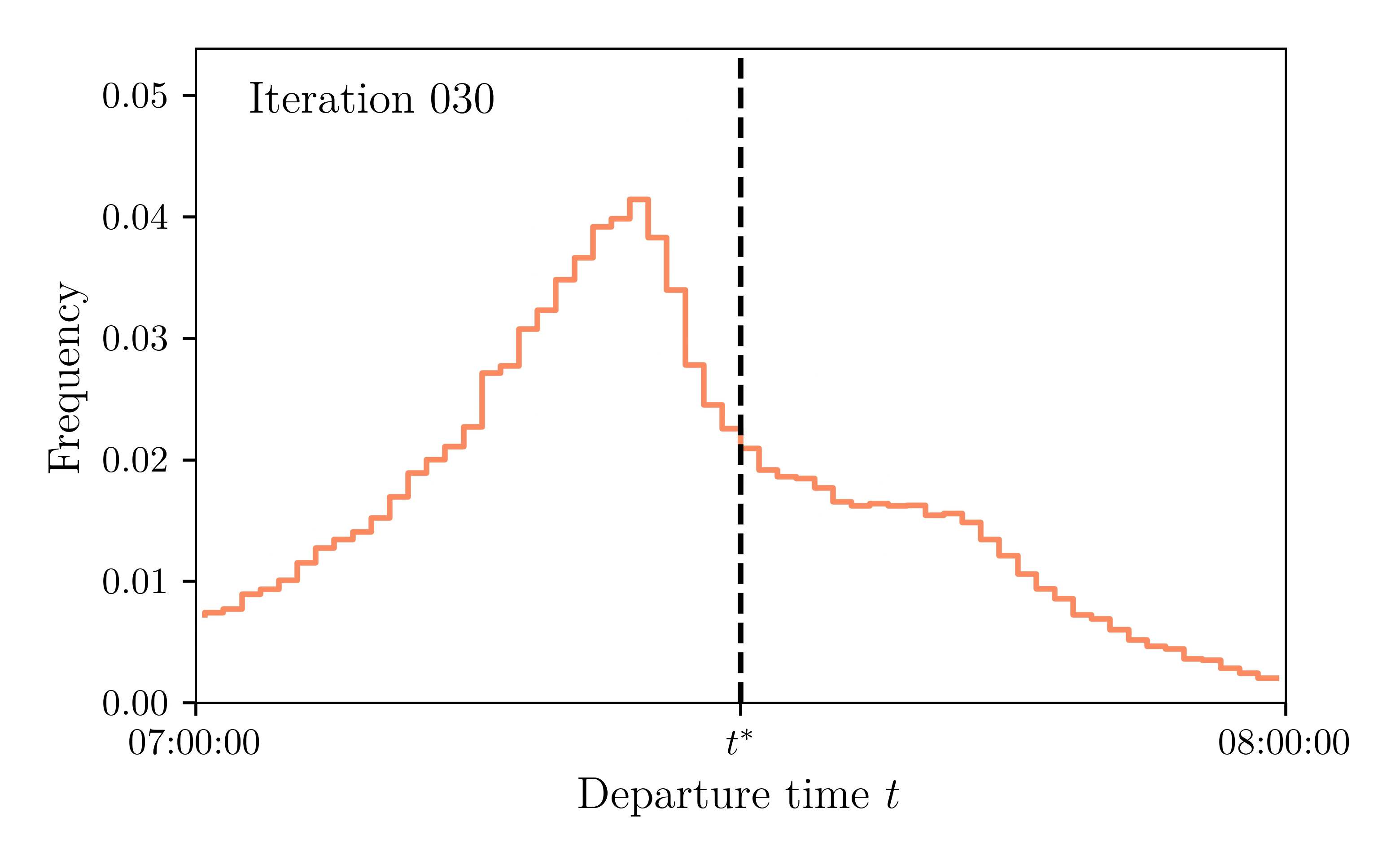
Departure rate: Iteration 30 & 31

Convergence Video
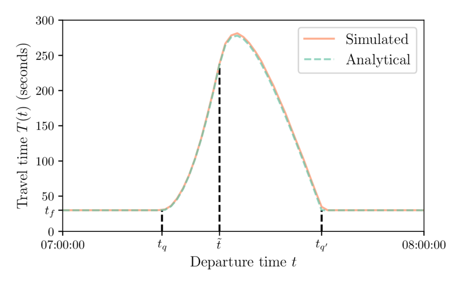
Comparison to Analytical Results
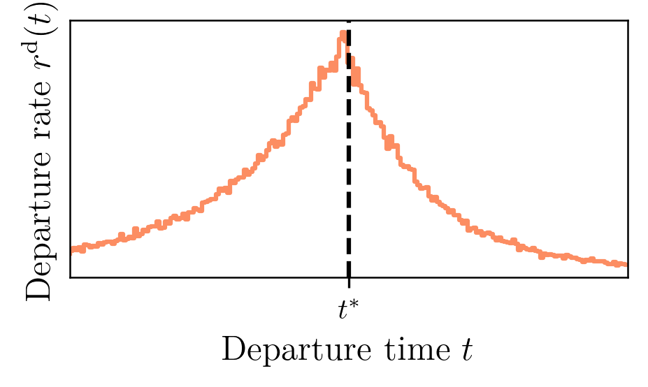
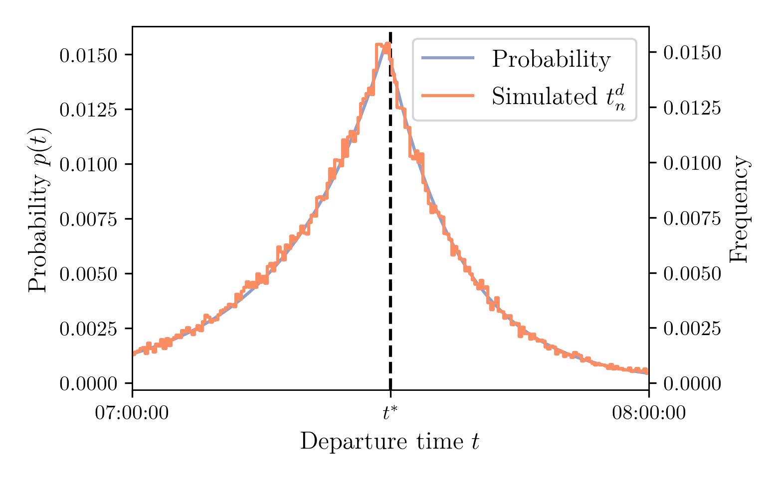
Departure-time distribution
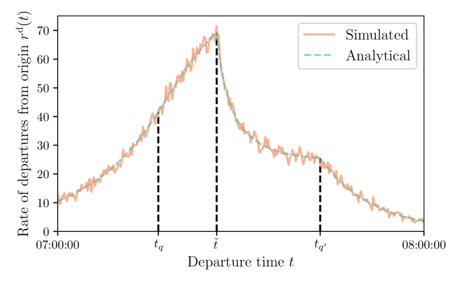
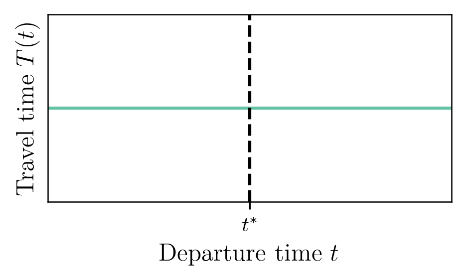
Travel-time function
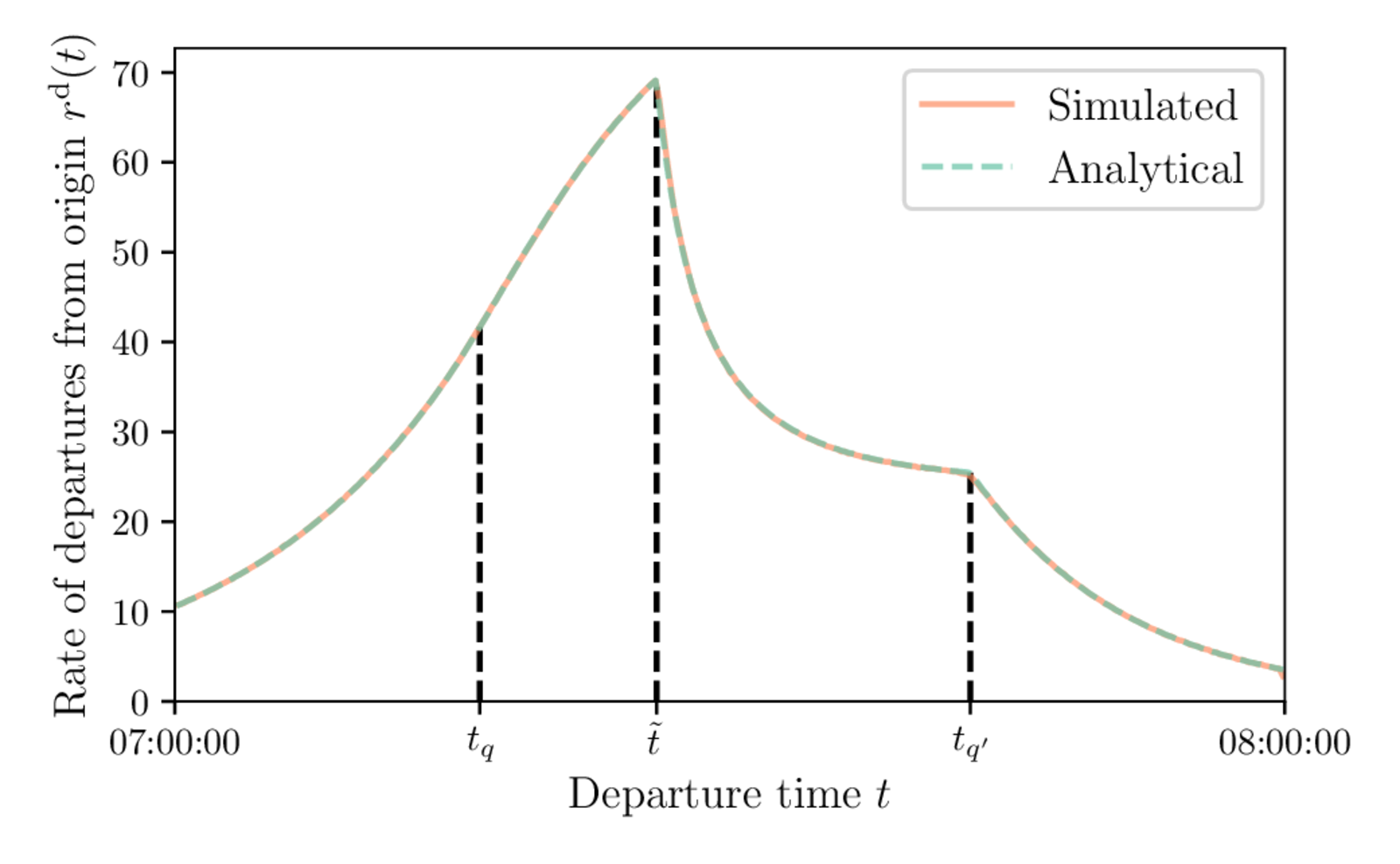
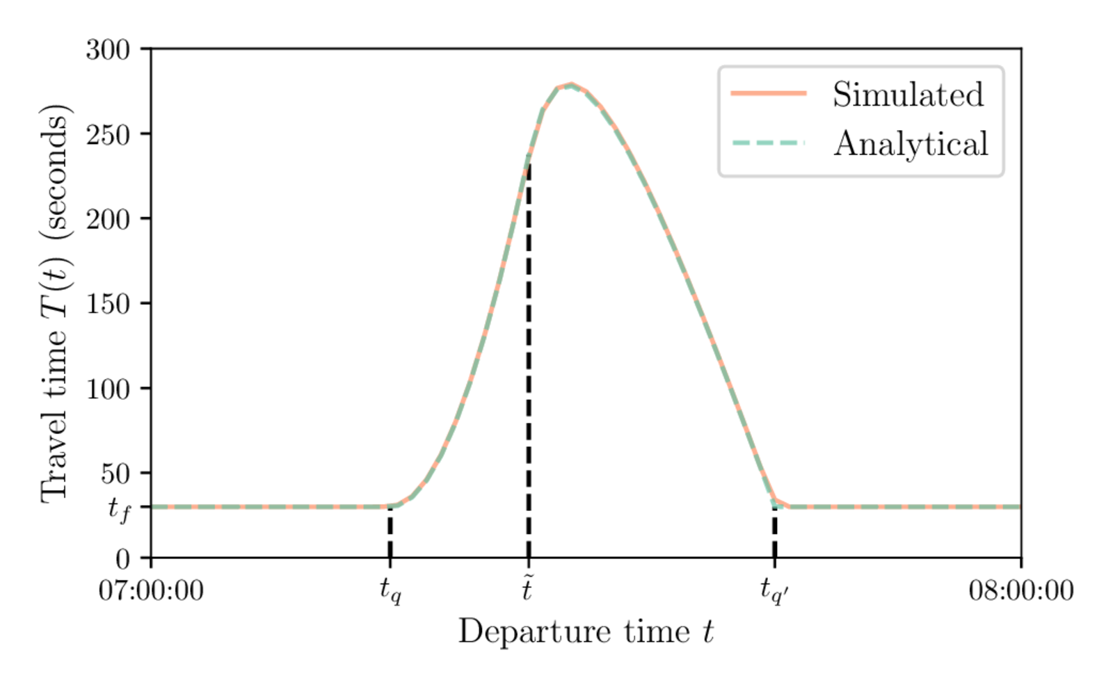
Systematic Sampling
Systematic sampling: using evenly spaced values in $[0, 1]$ instead of random draws
Departure-time distribution
Travel-time function
METROPOLIS2: Large-Scale Supply Side
- Road network: arbitrary graph of nodes (intersections) and edges (road links)
- Congestion: link-level bottleneck and speed-density function, queue propagation (spillback)
- Vehicle types: headway, speed limits, road restrictions
METROPOLIS2: Large-Scale Demand Side
- Mode choice: arbitrary number of modes (congested and uncongested)
- Route choice: fastest route computed with a routing algorithm (Contraction hierarchies)
- Trip chaining: arbitrary number of trips with exogenous activity duration
- Utility function: function of travel time, departure time, arrival time
Example Application: Paris' Urban Area
| METROPOLIS1 | METROPOLIS2 | |
|---|---|---|
| Running time | 18h 29m | 1h 49m |
| RMSE departure time | 2m 5s | 5s |
| Average utility | -5.58 € | -5.32 € |
| Average travel time | 16m 23s | 15m 33s |
Conclusion
- We proposed a simulation methodology to solve some analytical models
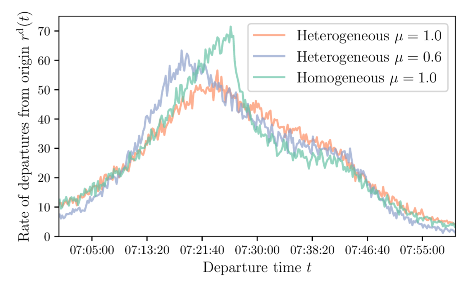
- The methodology can be used to solve models which are too complex to be derived analytically (e.g., toy network, heterogeneous $t^*$)
- The methodology can be extended into a large-scale transport simulator with good convergence and small distance to equilibrium
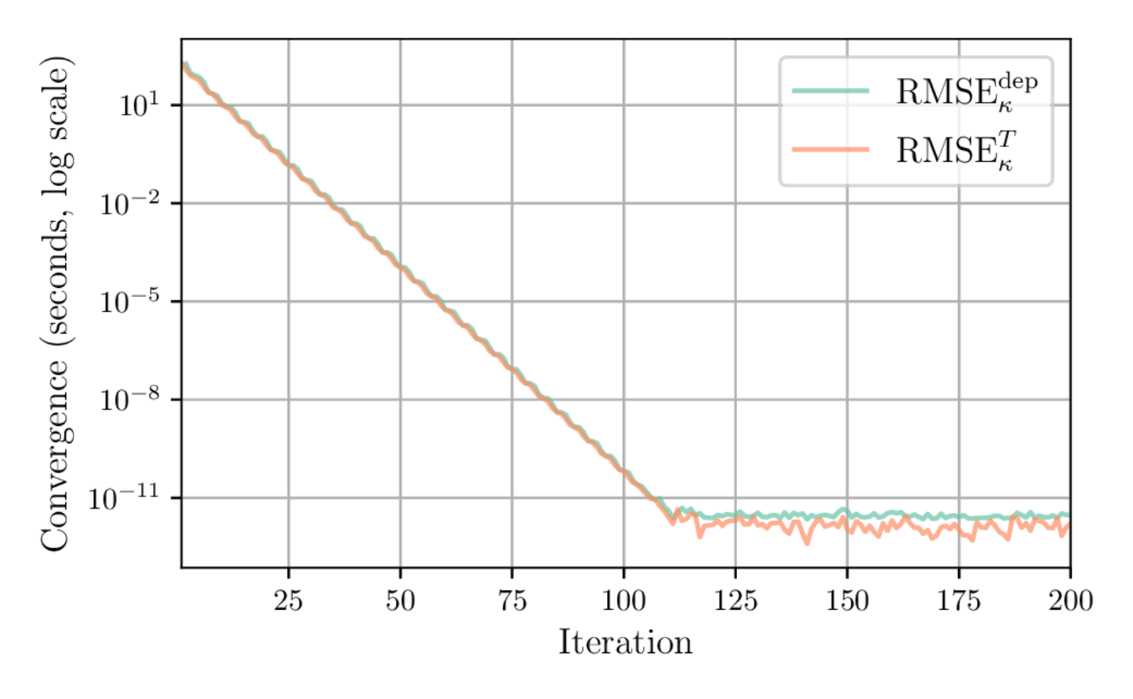
Convergence
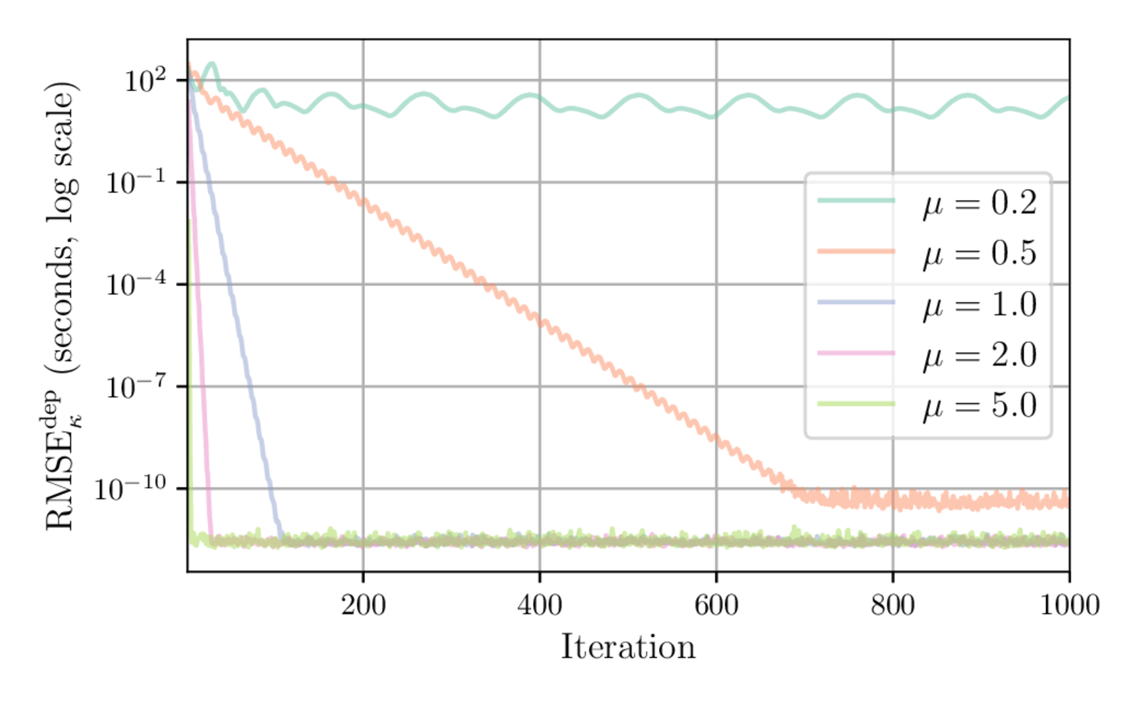
Impact of utility scale on convergence
Heterogeneous desired arrival times