METROPOLIS2 Course
Session 7: Output Side of Paris' Simulation
Lucas Javaudin
Spring 2024
Plan of this Session
- Pollution Emissions and Fuel Consumption
- Policy Evaluation
Required Data
- Road links' length → Imported OpenStreetMap road network
- Entry and exit time of agents on the road links of their itinerary → METROPOLIS2 output (
route_results.parquet) - Vehicle type for each agent → Household vehicles generated from municipality-level fleet data (See Session 6)
- Emission factors by pollutant and by vehicle type → See Romuald's presentation
Getting Started
- A Python script is available in the METROPOLIS2 Python library to compute a table of emissions by agent, by road link and by time period from the 4 input listed in the previous slide
- Indicators that can be computed: Nitrogen oxides (NOx), Carbon monoxide (CO), fine particulate matter (PM2.5), energy consumption
- Carbon dioxide (CO2) emissions (in grams) and fuel consumption (in grams) are also derived from energy consumption (in joules)
- Methodology: For each link taken by an agent, the average speed on the link is computed (from entry time, exit time and link length), then the emissions are computed based on the average speed, the agent's vehicle type (European emission standard) and the emission factors
Emissions by Agent
NOx emissions by agent as a function of the trip length
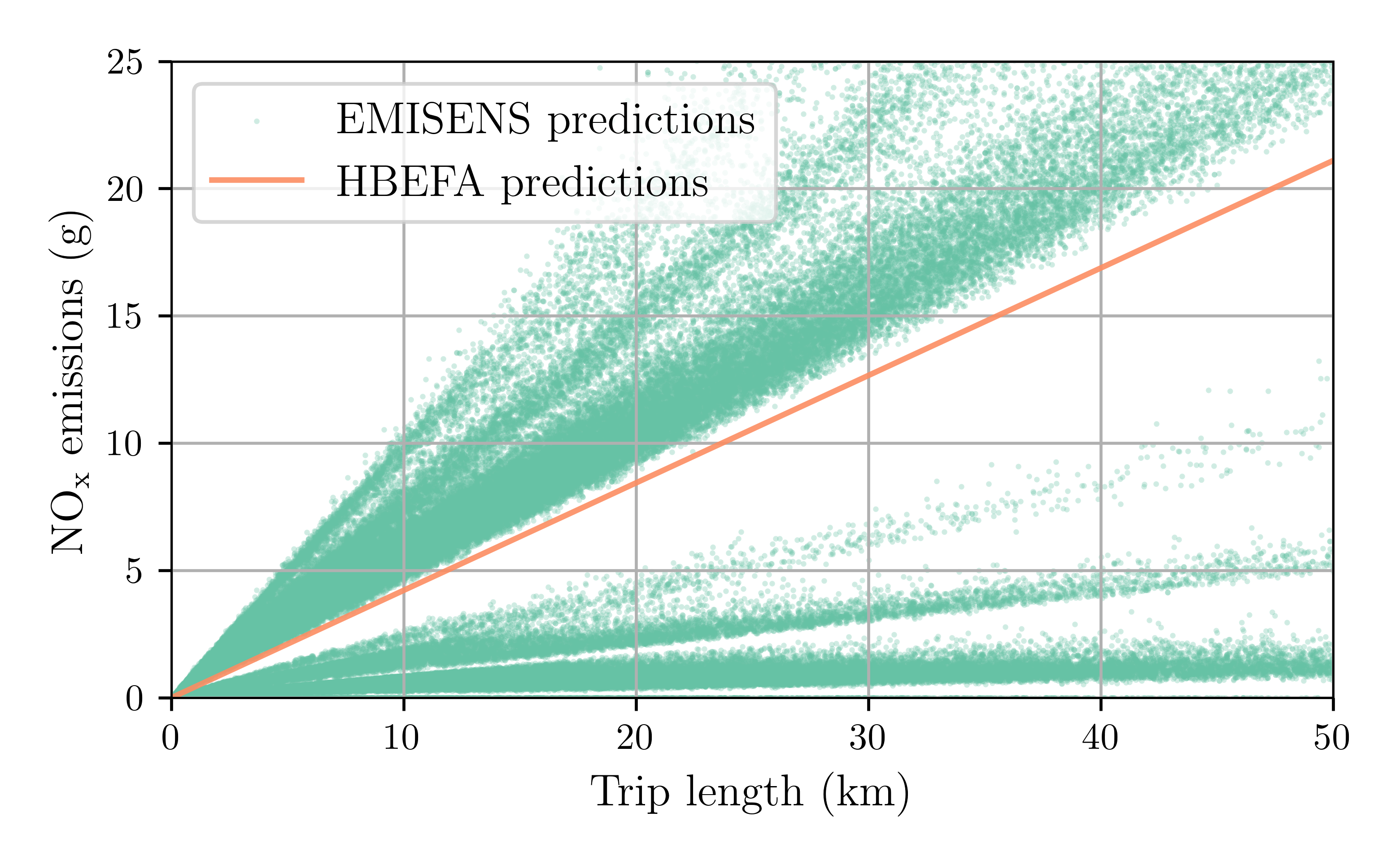
The various vehicle types are clearly visible
Emissions by Agent
Average NOx emissions by agent in each IRIS zone
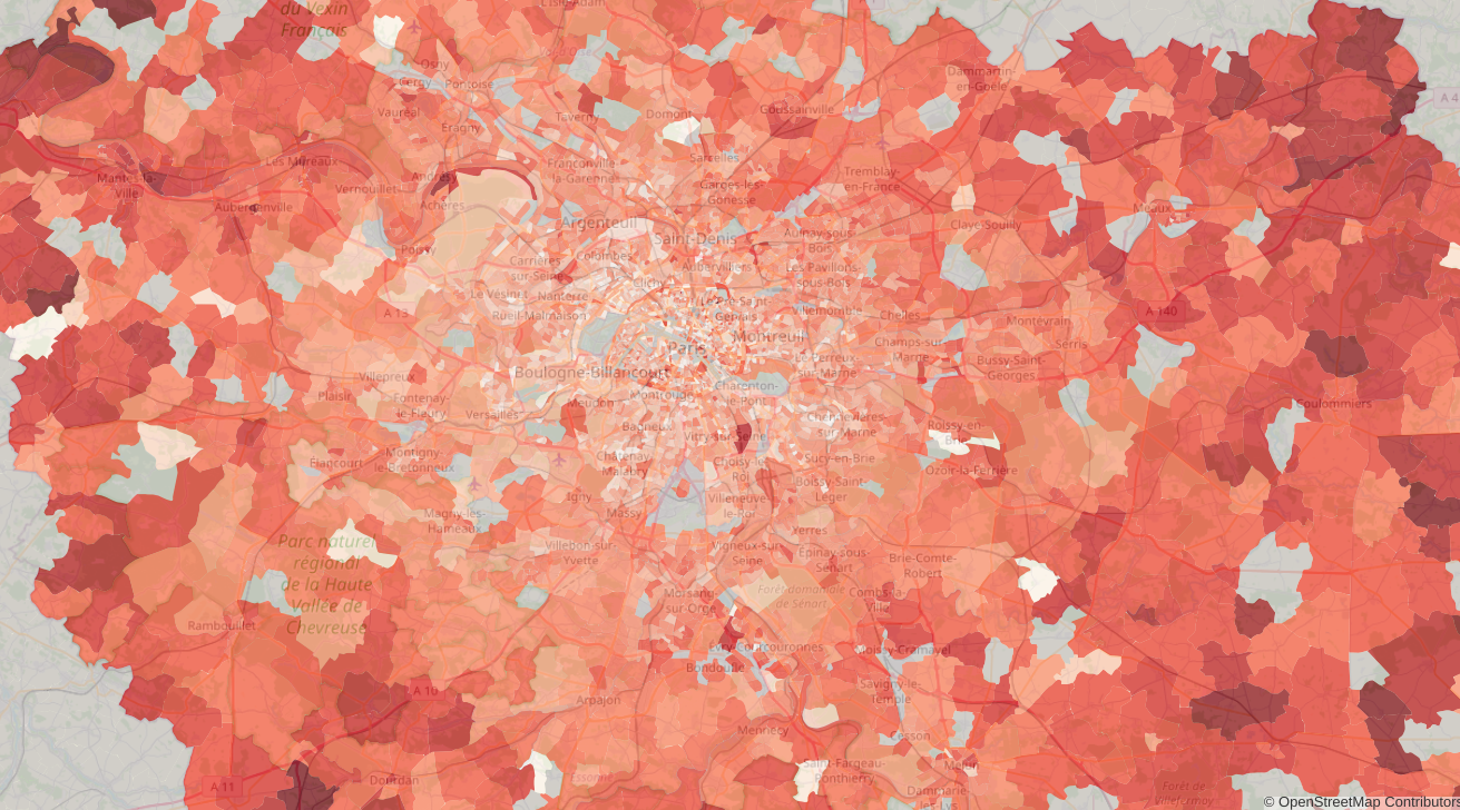
Agents living further away from Paris emit more NOx on average (they have longer trips)
Emissions by Road Link / Time Period
Total NOx emissions per meter by edge
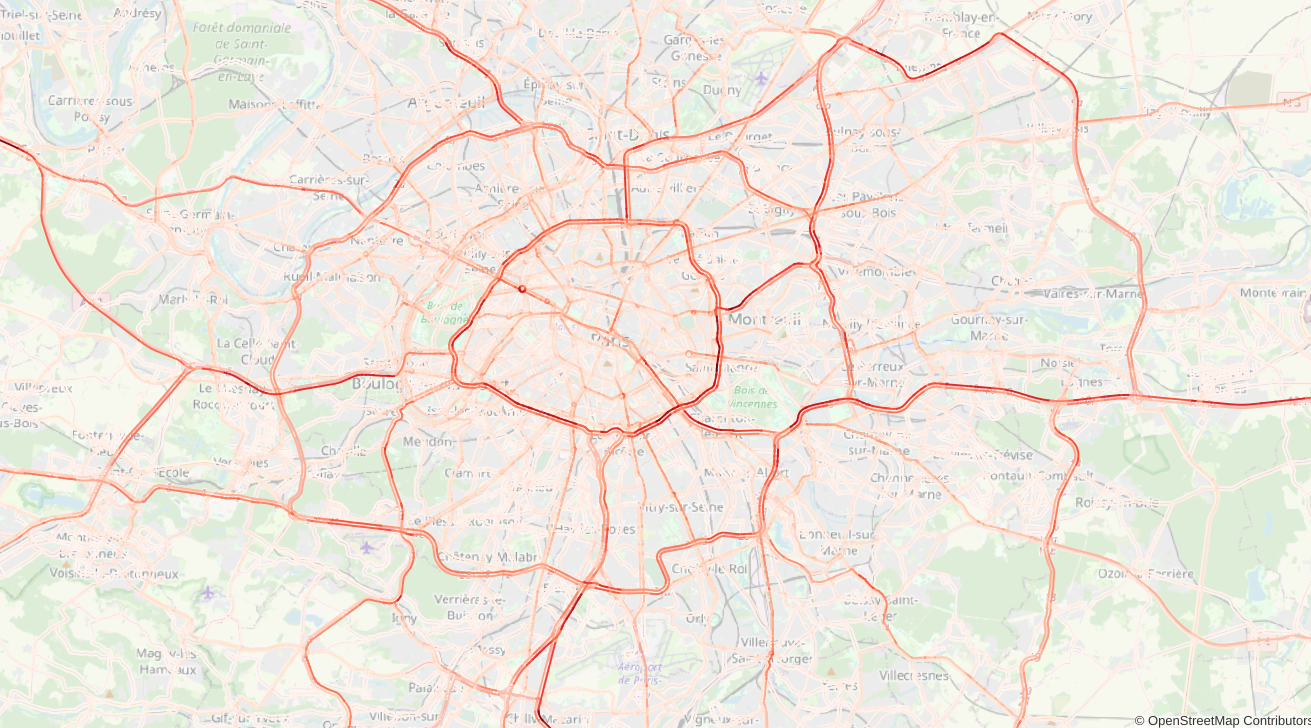
Emissions are larger on the main ring road and arterial motorways (toward Paris)
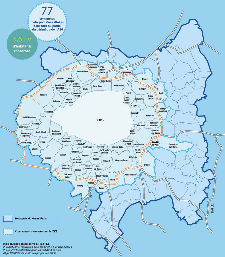
Case Study: Paris' Low Emission Zone
- More than 5 million inhabintants are living in the LEZ
- The LEZ represent around 10 % of the Île-de-France's road network
- June 2021: Crit'air 4 vehicles and worse are banned (11 % of the fleet)
- January 2025: Crit'air 3 vehicles and worse are banned (32 % of the fleet) [This is the policy evaluated in the following]
- 68 € fine for non-respect (traffic-camera ticketing is planned)

Policy Evaluation: Basic Principles
- Run two simulations: baseline (without policy) and counterfactual (with policy)
- Use the same random draws for the two simulations so that different choices are explained by the policy, not by different draws
-
Compare relevant indicators based on the policy evaluated:
- Low emission zone → air pollution, spatial and economic inequalities
- New public-transit line → mode share, travel time
- Cordon-area congestion pricing → travel time, spatial and economic inequalities
Examples of Indicators to Compare
Agent-level:
- Utility
- Travel time
- Schedule delay
- Fuel consumption
Externalities:
- Local pollution (NOx, CO, PM2.5)
- Global pollution (CO2)
Global / network-level:
- Mode shares
- Traffic flows
- Public-transit occupancy
Aggregate Comparison
Aggregate results can either be read directly from iteration_results.parquet or they can be computed from agent_results.parquet or trip_results.parquet
| Baseline | Counterfactual | Variation | |
|---|---|---|---|
| Car users | 2.101 M | 1.883 M | -10.4 % |
| Vehicle kilometers | 31.04 M km | 28.23 M km | -9.0 % |
| Travel time | 29m 24s | 30m 8s | +2.4 % |
| Congestion index | 29.40 % | 24.56 % | -16.5 % |
| Average travel surplus | 7.37 € | 7.25 € | -0.09 € |
Comparing Same Populations
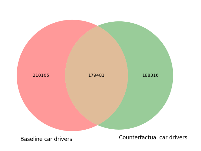
The red and green populations are not comparable
| Mean travel time baseline | Mean travel time counterfactual | Variation | |
|---|---|---|---|
| Agents traveling by car in the current scenario | 23m 7s (210,105) | 21m 44s (188,316) | -6.03 % |
| Agents traveling by car in both scenarios | 22m 18s (179,481) | 20m 49s (179,481) | -6.62 % |
Mode Shares Comparison
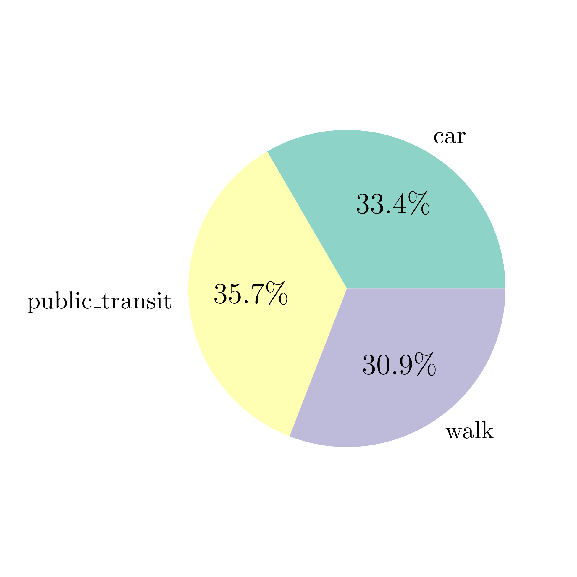
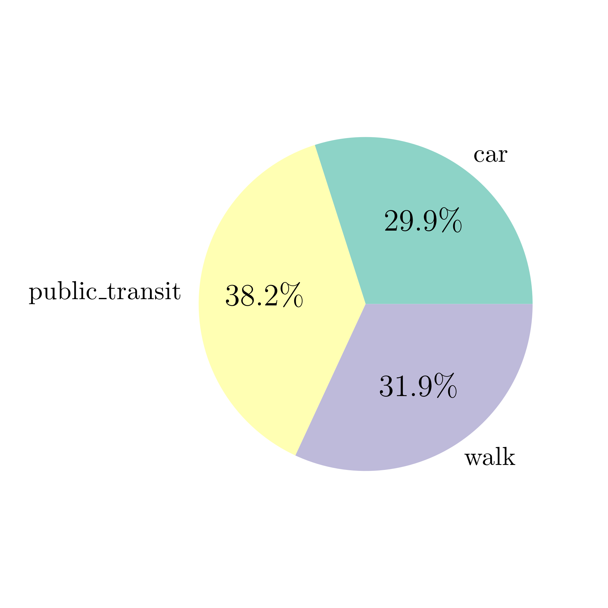
Aggregate mode shares do not tell the full story (e.g., is there a rebound effect?)...
Mode Shares Comparison
By comparing results at the agent-level, we are able to identify the mode shifts
Baseline Counterfactual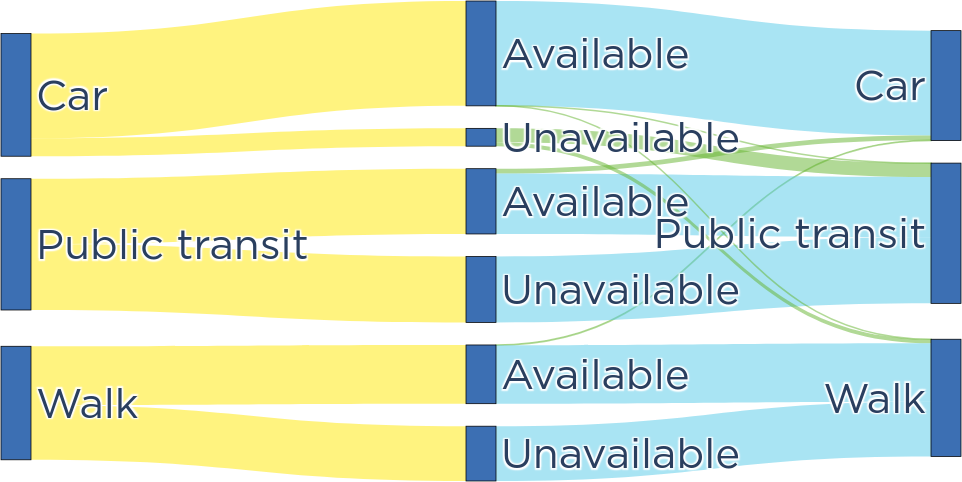
Available: authorized car is available
Unavailable: no car or only banned cars are available
Main shift: owners of banned cars drop their cars for public transit
Traffic Flow Comparison
From route_results.parquet, we can compute the flow of vehicles on any road link.
By comparing the two simulations, we can identify where the flows have increased or decreased.
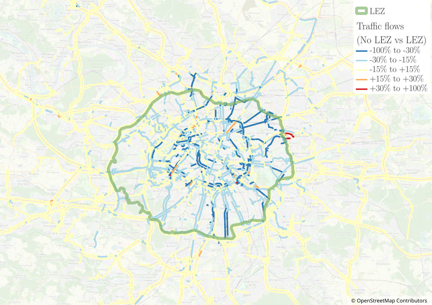
Traffic flows decrease almost exclusively inside the Low Emission Zone
Public-Transit Occupancy Comparison
From agent_results.parquet, we can retrieve the id of the agents who traveled by public transit and, from the OpenTripPlanner results, we know the itinerary that they took (see Session 6).
By comparing the two simulations, we can identify where the stop pairs where occupancy has increased or decreased.
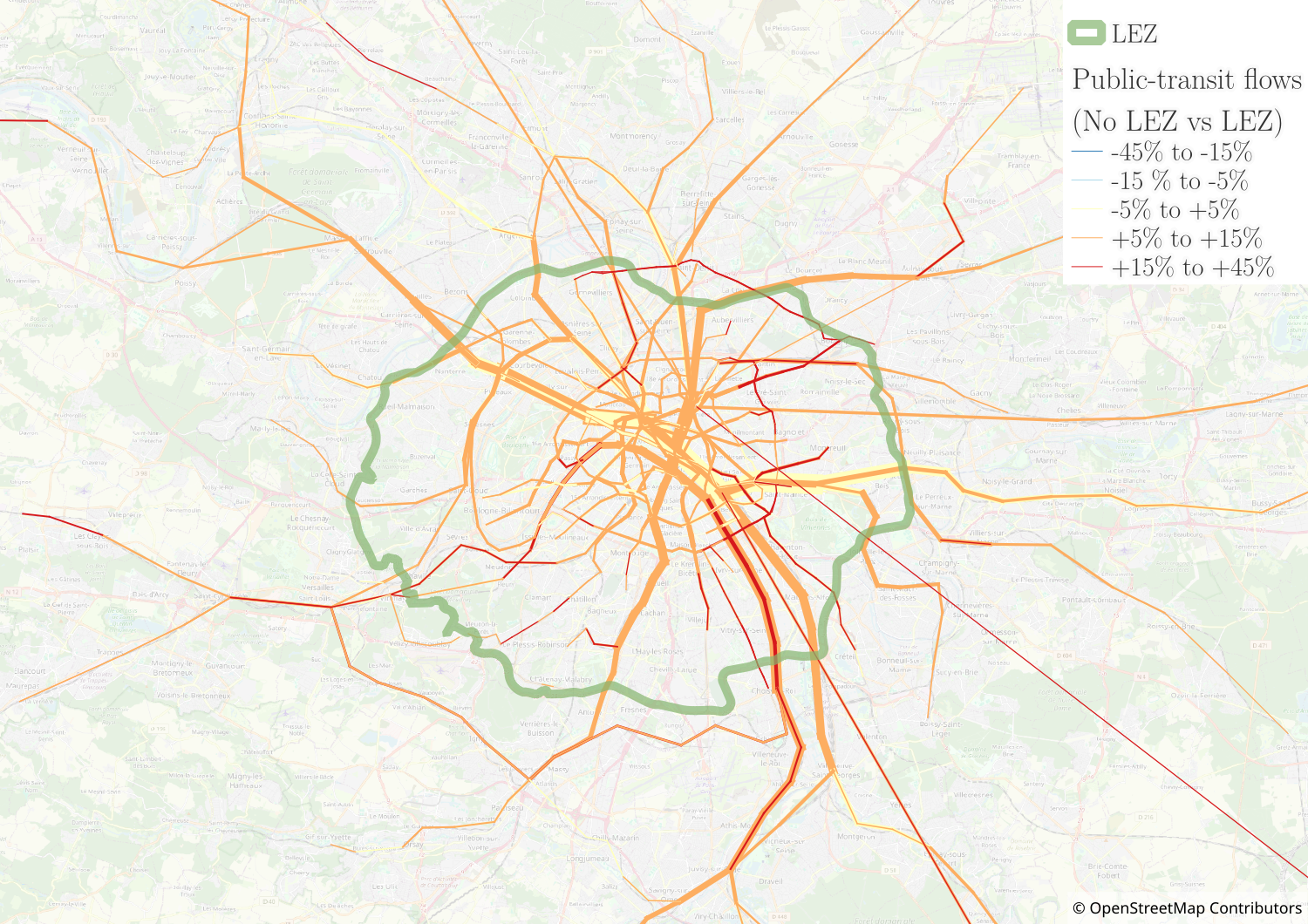
Occupancy increases for all main lines.
Population Segmentation
- To analyze results at the agent-level, it is easier to create population segments
-
Examples of segments:
- By sex
- By age
- By socio-professional category
- By car ownership (clean car vs banned car vs no car)
- By home municipality
- By income
- Warning: Some segment comparisons might not be valid (e.g., comparing poor vs rich agents in the LEZ application when cars are drawn independently of income)
Surplus by Car Ownership Segments
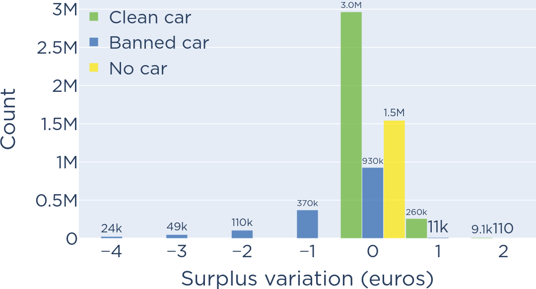
- No car: no impact, they keep the same mode (PT or walk) and have the same travel time
- Banned car owners: many negative impacts, they have to make a detour or switch mode
- Clean car owners: some positive impacts, they face less congestion during their car trips
Surplus by IRIS Zone
From the synthetic population, we know the home location of each agent so we can compute the average surplus by home IRIS zone and compare its variation from baseline to counterfactual.

- Inside the LEZ: mostly losers (banned cars cannot be used)
- Outside the LEZ: some losers (banned cars cannot be used to travel to the LEZ) and some winners (less congestion)
Surplus by Municipality Income
It is not correct to compare surplus variation by income at the agent-level in this application.
Instead, we can compare surplus variation by income at the municipality-level (the car fleet is valid at the municipality-level).
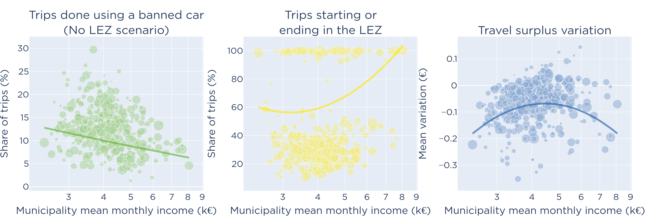
- Travel surplus variation inside a municipality can be explained by two opposing effects
- Banned-car-use effect: Poorest municipalities are using banned cars more often
- Traveling-to-LEZ effect: Richest municipalities are traveling from / to the LEZ more often (they are closer to the LEZ)
- Global effect: Poorest and richest municipalities are loosing the most in travel surplus from the LEZ
Comparing Indicators Together
- Comparing indicators in the baseline and counterfactual tells us the impact of the policy on various aspects (e.g., mode shares, travel surplus, air pollution)
- How to tell whether the positive effect on air quality overcome the negative effect on travel surplus? → Cost-Benefit Analysis
- Basic principle: convert all indicators to monetary value so that they can be compared
Conversion to Monetary Value
-
Expected utility / surplus:
- Utility is expressed in monetary value as long as both all the parameters (value of time, utility constant, early / late schedule-delay penalty, etc.) are expressed in monetary value themselves
- Utility is usually defined "up-to a constant" (the utility of an alternative is normalized to zero) so the average surplus cannot be interpreted directly (i.e., an average surplus of -4 euros does not really mean anything)
- When comparing surplus between simulations, the normalization constant "disappears" so the difference of surplus can be interpreted (e.g., from baseline to counterfactual, the average surplus decreases by 9 cents)
Conversion to Monetary Value
- CO2: Use standard value for social cost of carbon (e.g., 100 euros per ton of CO2)
-
Air pollution: three options
- Give monetary value to vehicle-kilometers (e.g., French recommended values: 1.3 euros per 100 vehicle-kilometers in urban areas)
- Give monetary value to the quantity of pollutants emitted (Handbook on the External Costs of Transport, Delft)
- Give monetary value for exposure to pollution (METRO-TRACE: Le Frioux, de Palma, Blond, 2023)

Cost-Benefit Analysis
After conversion to monetary values, the values can be aggregated in a table of costs and benefits, with a global indicator of the policy impact.
| Travel surplus | - 565 k € | |
| inc. owners of banned cars | - 1 010 k € | |
| inc. owners of clean cars | + 445 k € | |
| Health surplus | + 18 052 k € | |
| inc. exposure to NOx | + 15 616 k € | |
| inc. exposure to PM2.5 | + 2 080 k € | |
| inc. exposure to CO | + 356 k € | |
| Environmental surplus (200 € / ton CO2) | + 95 k € | |
| Global impact | + 17 582 k € |
|---|
Disclaimer: Provisional results