METROPOLIS2 Course
Session 5: Simulation Output
Lucas Javaudin
Spring 2024
Output Files
log.txt: METROPOLIS2 log messages during the simulationrunning_times.json: simulation running time, by categoryreport.html: webpage summarizing the resultsiteration_results.{parquet,csv}: aggregate results for each iteration- 3 CSV / Parquet output files for the population results
- 4 CSV / Parquet output files for the road-network results
Plan of this Session
- Aggregate Results
- Population Results
- Road-Network Results
- Task for Next Session
Running times (1/3)
File running_times.json
						{
							"total": "49181.060006808",
							"total_skims_computation": "37804.951886765",
							"total_demand_model": "2943.497363545",
							"total_supply_model": "8150.961492634",
							"total_learning_model": "9.425217904",
							"total_aggregate_results_computation": "148.839589353",
							"total_stopping_rules_check": "0.000029886",
							"per_iteration": "245.905300034",
							"per_iteration_skims_computation": "189.024759433",
							"per_iteration_demand_model": "14.717486817",
							"per_iteration_supply_model": "40.754807463",
							"per_iteration_learning_model": "0.047126089",
							"per_iteration_aggregate_results_computation": "0.744197946",
							"per_iteration_stopping_rules_check": "0.000000149"
						}
skims_computation: computation of OD-level travel-time functions given the expected road-network conditions
Running times (2/3)
Impact of simulation size on running times:
| Skims comp. | Demand model | Supply model | |
|---|---|---|---|
| # agents | · | Large¹ | Large¹ |
| # nodes / edges | Large | · | Medium |
| # unique origin / dest. | Very large | · | · |
| # unique OD pairs | Large | · | · |
| # breakpoints | Small | Very small | Very small |
¹: A priori, the number of agents increases linearly the running time of the demand and supply models but, if congestion is larger, the global running time gets larger.
Running times (3/3)
Comparing two Paris simulations
| Old scenario | New scenario | Variation | |
|---|---|---|---|
| # agents | 477 192 | 629 314 | ×1.32 |
| # road trips | 477 192 | 548 480 | ×1.15 |
| # virtual trips | 0 | 1 442 883 | ×∞ |
| # nodes | 20 648 | 116 971 | ×5.67 |
| # edges | 43 857 | 196 980 | ×4.49 |
| # unique origins | 1326 | 50 774 | ×38.29 |
| # unique destinations | 1326 | 49 607 | ×37.41 |
| # unique OD pairs | 161 871 | 466 079 | ×2.88 |
| # breakpoints | 27 | 93 | ×3.44 |
| Old scenario | New scenario | Variation | |
|---|---|---|---|
| Total | 01:49:42 | 09:00:28 | ×4.93 |
| Skims computation | 00:20:04 | 06:57:25 | ×20.80 |
| Demand model | 00:44:43 | 00:39:28 | ×0.88 |
| Supply model | 00:42:35 | 01:19:11 | ×1.86 |
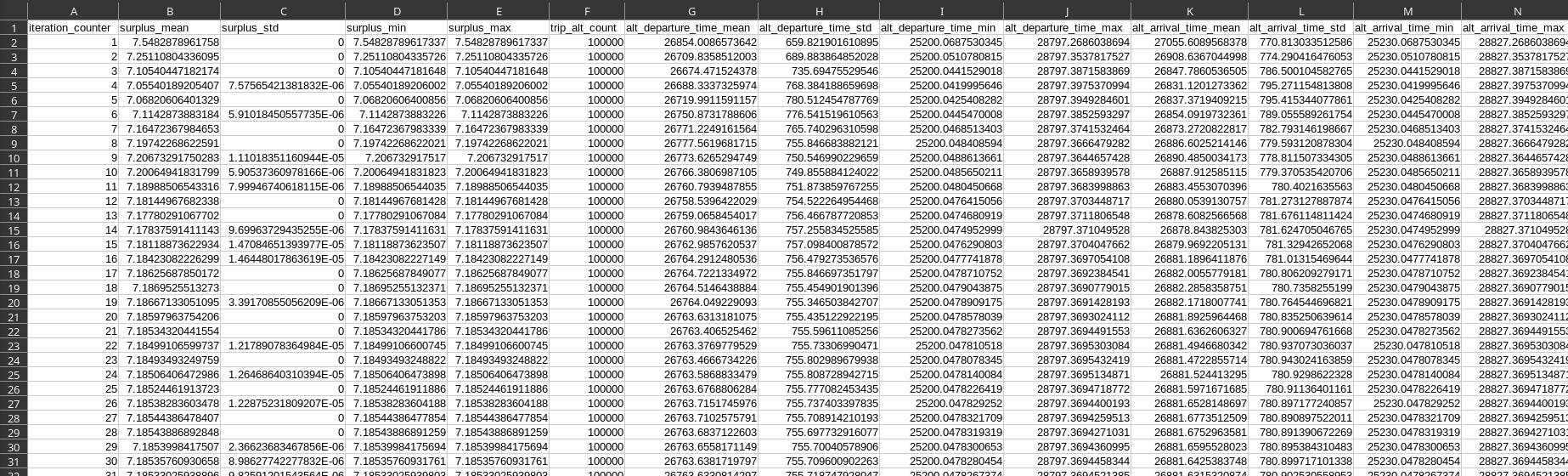
HTML Report
- Table of aggregate results by iterations
- Graphs of convergence through iterations
- Graphs of departure-time / arrival-time distribution for last iteration
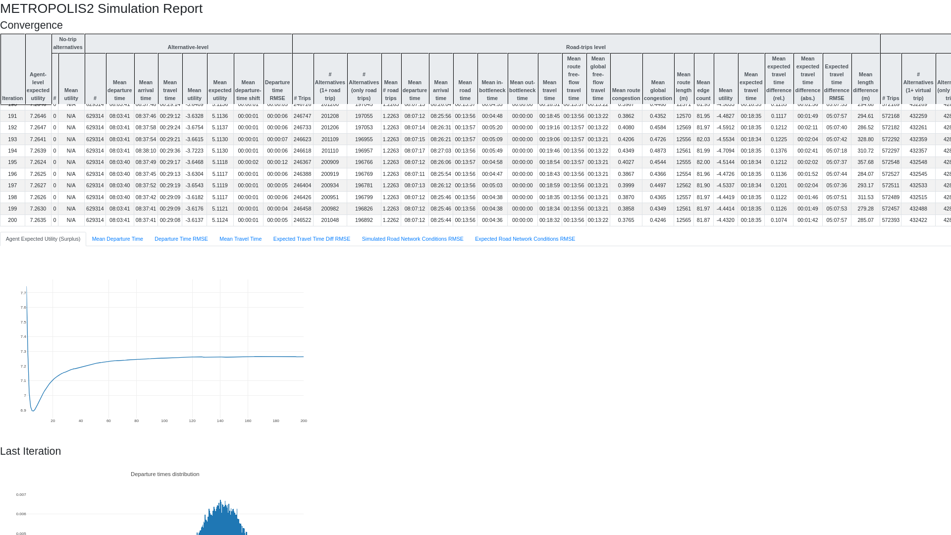
Iteration Results
- Parquet or CSV file
- 1 row for each iteration; 145 columns
- Aggregate results at the agent-level, road-trip level, virtual-trip level and road-network level
- Same variables as in the HTML report (with standard-deviation, minimum and maximum)
Route vs Global Free-Flow Travel Time
- Route free-flow travel time: no-congestion travel time on the route that was taken
- Global free-flow travel time: no-congestion travel time on the fastest possible route
- Route / Global congestion: share of travel-time spent in congestion, relative to route / global free-flow travel time
Output Files
All the results are specific to the last iteration
agent_results.{parquet,csv}: results at the agent-leveltrip_results.{parquet,csv}: results at the trip-levelroute_results.{parquet,csv}: detailed itineraries for the road trips
Agent Results
- Parquet or CSV file
- 1 row for each agent; 12 columns
- Results specific to the agents and their selected alternative
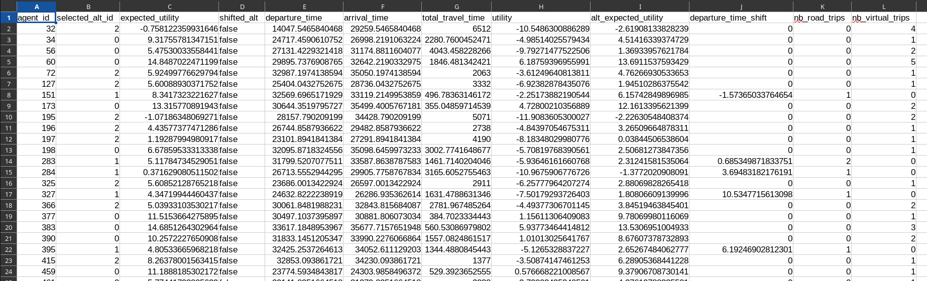
Utility Indicators (1/4)
-
utility: Simulated utility, based on the selected alternative $j$ and departure time $\tau$: $V^{\text{sim}}_{j}(\tau)$ -
alt_expected_utility: Expected utility of the departure-time choice of the selected alternative $j$: $\mathbb{E}_{\varepsilon}[\max_{\tau} U_j(\tau)]$ -
expected_utility: Expected utility of the alternative choice: $\mathbb{E}_{\varepsilon}[\max_{j} U_j]$
Utility Indicators (2/4)
Example with a deterministic alternative-choice model and a constant departure time
-
utility: Simulated utility, based on the selected alternative $j$, departure time $\tau$ and simulated travel times: $V^{\text{sim}}_{j}(\tau)$ -
alt_expected_utility: Expected utility, based on the selected alternative $j$, departure time $\tau$ and expected travel times: $V^{\text{exp}}_{j}(\tau)$ -
expected_utility: Expected utility, based on the selected alternative $j$, departure time $\tau$ and expected travel times: $V^{\text{exp}}_{j}(\tau)$
When the simulation has converged: $V^{\text{sim}}_j(\tau) \approx V^{\text{exp}}_j(\tau)$
Utility Indicators (3/4)
Example with a Logit alternative-choice model and a Continuous Logit departure-time choice model
-
utility: Simulated utility, based on the selected alternative $j$, departure time $\tau$ and simulated travel times: $V^{\text{sim}}_{j}(\tau)$ -
alt_expected_utility: Logsum of departure-time choice for the selected alternative $j$ \[ \bar{U}_j \equiv \mathbb{E}_{\varepsilon}[\max_\tau U_j(\tau)] = \mu \ln \int_{t^0}^{t^1} e^{V_j^{\text{exp}}(\tau) / \mu} \text{d} \tau + \mu \cdot 0.577 \] -
expected_utility: Logsum of alternative choice ("logsum of logsum") \[ \mathbb{E}_{\varepsilon}[\max_j U_j] = \mu \ln \sum_j e^{\bar{U}_j / \mu} + \mu \cdot 0.577 \]
Utility Indicators (4/4)
Which one to use (e.g., for cost-benefit analysis)?
-
utility: not really adapted when using random-utility models (the random perturbations $\varepsilon$ are omitted); recommended when using deterministic models (including models with drawn epsilons) -
alt_expected_utility: intermediate indicator, useful in some special cases only expected_utility: recommended when using random-utility models (it depends on the range of alternatives available, not just the realized choice: two identical agents always have the sameexpected_utilitybut they can have differentutilityif their uniform draws differ)
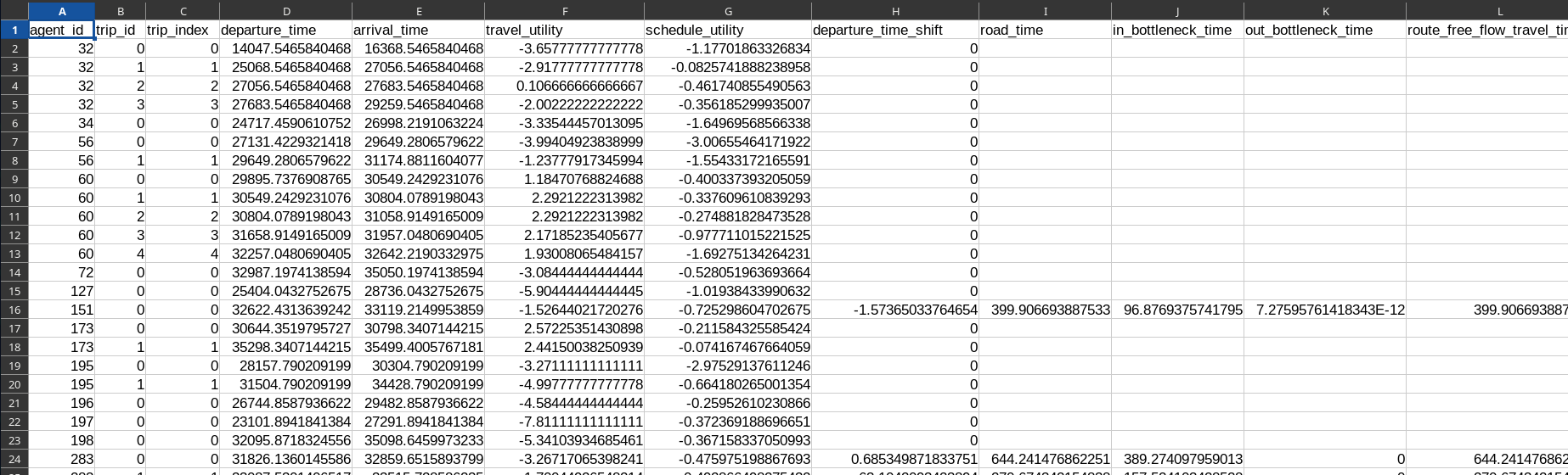
Trip Results
- Parquet or CSV file
- 1 row for each selected trip (road or virtual); 19 columns
- 11 columns are specific to road trips
Route Results
- Parquet or CSV file
- 1 row for each edge taken during road trips; 6 columns
- Detailed itinerary followed by the agents, as a list of edges with entry and exit time
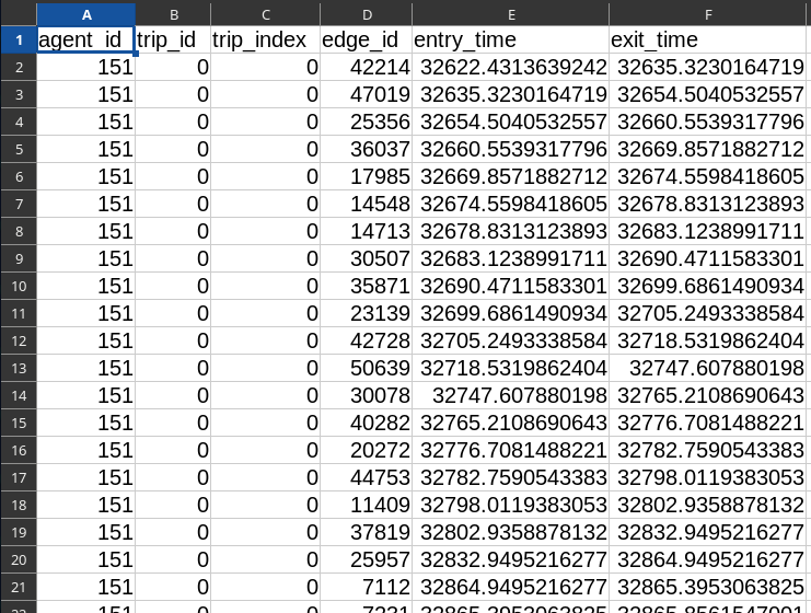
Route Results
Theroute_results.{csv,parquet} output file allows to show the detailed itinerary of an agent.
Route Results
Theroute_results.{csv,parquet} output file allows to show a video of the vehicle movements.
Output Files
Three files for the road-network conditions (edge-level travel-time functions):
net_cond_sim_edge_ttfs.{parquet,csv}: last iteration, simulatednet_cond_exp_edge_ttfs.{parquet,csv}: last iteration, expectednet_cond_next_exp_edge_ttfs.{parquet,csv}: next iteration, expected
One extra file:
skim_results.json.zst: OD-level (expected) travel-time functions
METROPOLIS2 Fundamental Flow Diagram
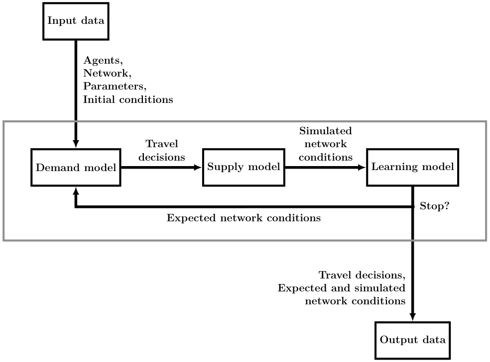
Network Conditions
- The network conditions consist in a travel-time function for each link and for each vehicle type
- The travel-time functions are represented as piecewise-linear functions with a fixed interval $\delta$ between two breakpoints
- Simulated network conditions: Network conditions observed, given some travel decisions (from the supply model).
- Expected network conditions: Network conditions anticipated by the agents when taking travel decisions (in the demand model). They are used to compute road trips' travel times.

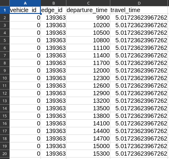
Network Conditions File Format
- Parquet or CSV file
- Number of rows: # edges × # breakpoints × # vehicle types
- Departure-time and travel-time breakpoints for each edge and vehicle type
- Departure-time breakpoints with simulated period [6 a.m., 10 a.m.] and recording interval 20 min.: [06:00, 06:20, 06:40, 07:00, 07:20, ..., 09:20, 09:40, 10:00]
Network Conditions Map
When merged with the edges' geometries, the network conditions can be plotted on a map.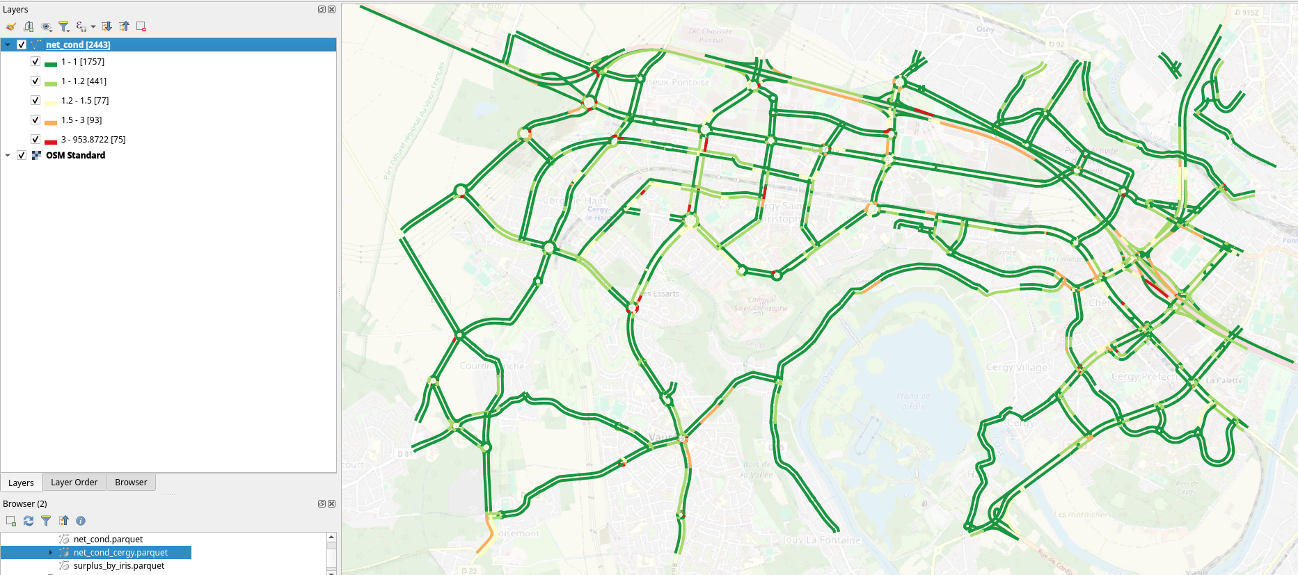
Starting Simulation from Network Conditions
- Default: use free-flow conditions as expected network conditions for the first iteration
- Initial network conditions can be given as input
- Input file format is the same as network conditions output file format
						{
								"input_files": {
										"agents": "agents.csv",
										"alternatives": "alts.csv",
										"trips": "trips.csv",
										"edges": "edges.csv",
										"vehicle_types": "vehicles.csv",
										"road_network_conditions": "net_cond_next_exp_edge_ttfs.csv"
								},
								"output_directory": "output",
								"period": [
										25200.0,
										28800.0
								],
								"road_network": {
										"recording_interval": 60.0,
										"spillback": false,
										"max_pending_duration": 0.0
								},
								"max_iterations": 100,
								"init_iteration_counter": 100,
								"saving_format": "CSV",
								"learning_model": {
										"type": "Exponential",
										"value": 0.4
								}
						}
parameters.json
Skim Results
- Travel-time function for each origin-destination pair in the population input (road trips)
- The travel-time functions are the one used in the demand model for the last iteration
- File format: compressed JSON for now; Parquet or CSV in a future update
Session 5 Task
From the results of your simulation (Task of Session 4), create some relevant graphs (e.g., travel-time distribution, travel utility vs schedule utility as a function of departure times) or maps (e.g., congestion on links as a function of time, link flows).