METROPOLIS2 Course
Session 4: Equilibrium and Convergence
Lucas Javaudin
Spring 2024
Plan of this Session
- Back to the Bottleneck Simulation
- Learning Model
- Convergence
- Task for Next Session
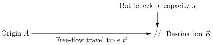
Edge File
Single road with a free-flow travel time of 30 seconds and a bottleneck with capacity 150 000 cars / hour.
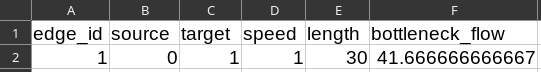
Vehicle-Type File
Single vehicle type: "car" with headway 1m and 1 PCE
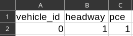
Agents File
- 150 000 agents
- No alternative choice (only one alternative per agent)
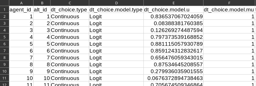
Alternatives File
- 150 000 alternatives (one per agent)
- Departure-time choice: Continuous Logit ($\mu = 1$)
- Utility function: \[ V(t^{\text{d}}, t^{\text{a}}) = - \alpha (t^{\text{a}} - t^{\text{d}}) - \beta [t^* - t^{\text{a}}]_+ - \gamma [t^{\text{a}} - t^*]_+ \] with $\alpha = 10 \$ / h$, $\beta = 5 \$ / h$, $\gamma = 7 \$ / h$ and $t^* =$ 7:30 a.m.
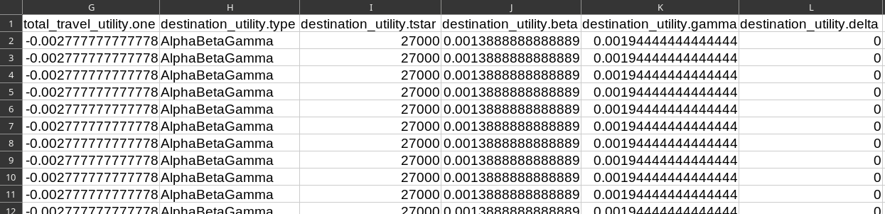
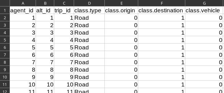
Trips File
- 150 000 trips (one per agent / alternative)
- Trip is a road trip from node $A$ (id 0) to node $B$ (id 1), with vehicle type "car" (id 0)
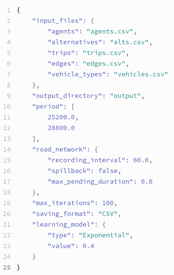
Parameters
- Simulated period: [7 a.m., 8 a.m.]
- Interval between two breakpoints in the travel-time functions: 60s
- Spillback is disabled
- 100 iterations
- Exponential learning model with $λ = 40\%$
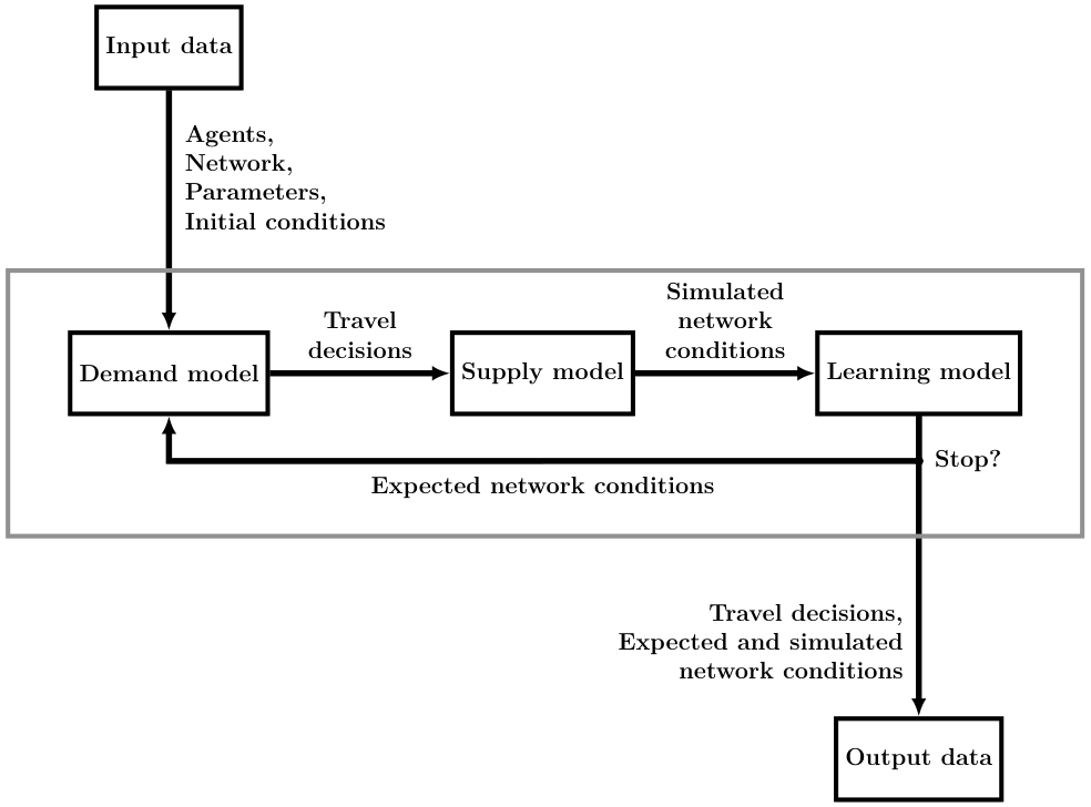
METROPOLIS2 Fundamental Flow Diagram
Network Conditions
- The network conditions consist in a travel-time function for each link and for each vehicle type
- The travel-time functions are represented as piecewise-linear functions with a fixed interval $\delta$ between two breakpoints
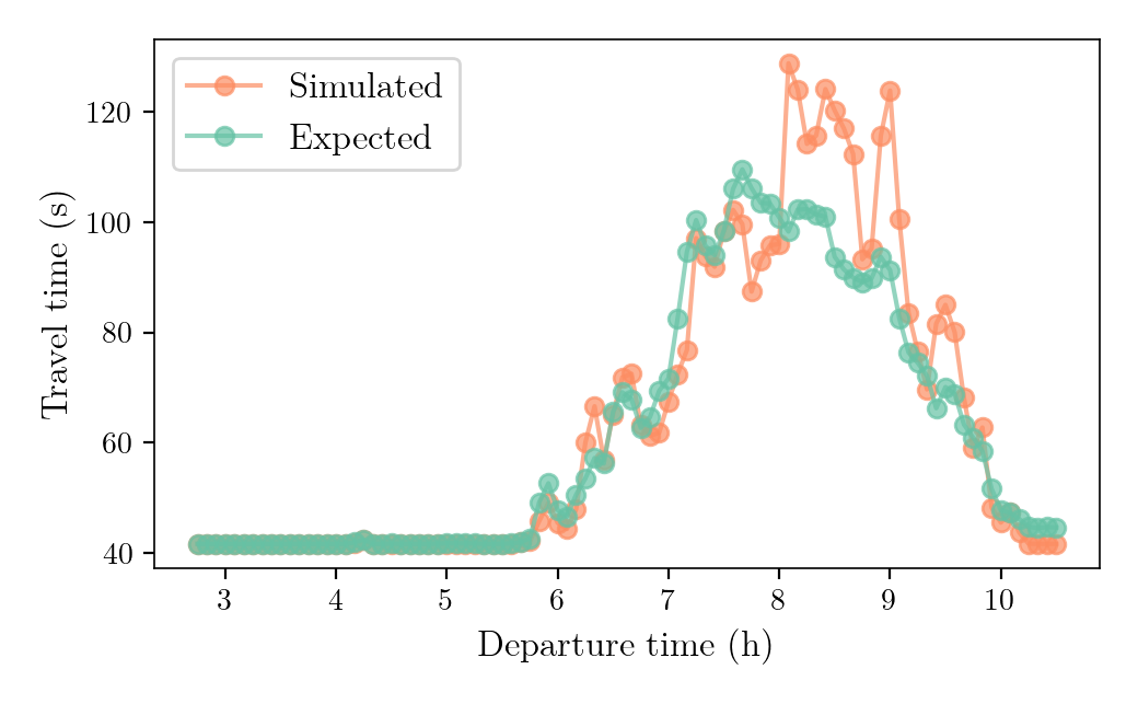
- Simulated network conditions: Network conditions observed, given some travel decisions (from the supply model).
- Expected network conditions: Network conditions anticipated by the agents when taking travel decisions (in the demand model). They are used to compute road trips' travel times.
- Both simulated and expected network conditions are common knowledge to all agents.

Learning Model
- The expected network conditions for the next iteration, $\mathbf{\hat{T}}_{\kappa+1}$, depends on the simulated network conditions, $\mathbf{T}_{\kappa}$ and the expected network conditions, $\mathbf{\hat{T}}_{\kappa}$, of the current iteration.
- At iteration $\kappa$: \[ \mathbf{\hat{T}}_{\kappa + 1} = f(\kappa, \mathbf{T}_{\kappa}, \mathbf{\hat{T}}_{\kappa}) \]
- Exponential smoothing method: \[ f(\kappa, \mathbf{T}_\kappa, \mathbf{\hat{T}}_{\kappa}) = \frac{\lambda}{\alpha_{\kappa}} \mathbf{T}_\kappa + (1 - \lambda) \frac{\alpha_{\kappa}}{\alpha_{\kappa+1}} \mathbf{\hat{T}}_{\kappa} \] with $\lambda \in [0, 1]$, the smoothing factor.
- With $\lambda = 1$: "naive" learning; with $\lambda = 0$: arithmetic mean.
- Other learning functions are available and described in the documentation.
Equilibrium
- Goal of METROPOLIS2: Find a Nash equilibrium from the input data
- Nash equilibrium: No agent can improve their utility given the travel decisions of the other agents
- Informal definition: The expected network conditions when agents took their travel decisions are equal to the simulated network conditions from these travel decisions.
- Formal definition (fixed point problem): \[ f^{\text{demand}}(f^{\text{supply}}(\bar{\mathbf{z}}; \mathbf{D}); \mathbf{D}) = \bar{\mathbf{z}} \] $\mathbf{D}$: input data; $\bar{\mathbf{z}}$: equilibrium travel decisions
Recommendations
- Run METROPOLIS2 for a fixed number of iterations, then check the distance to an equilibrium
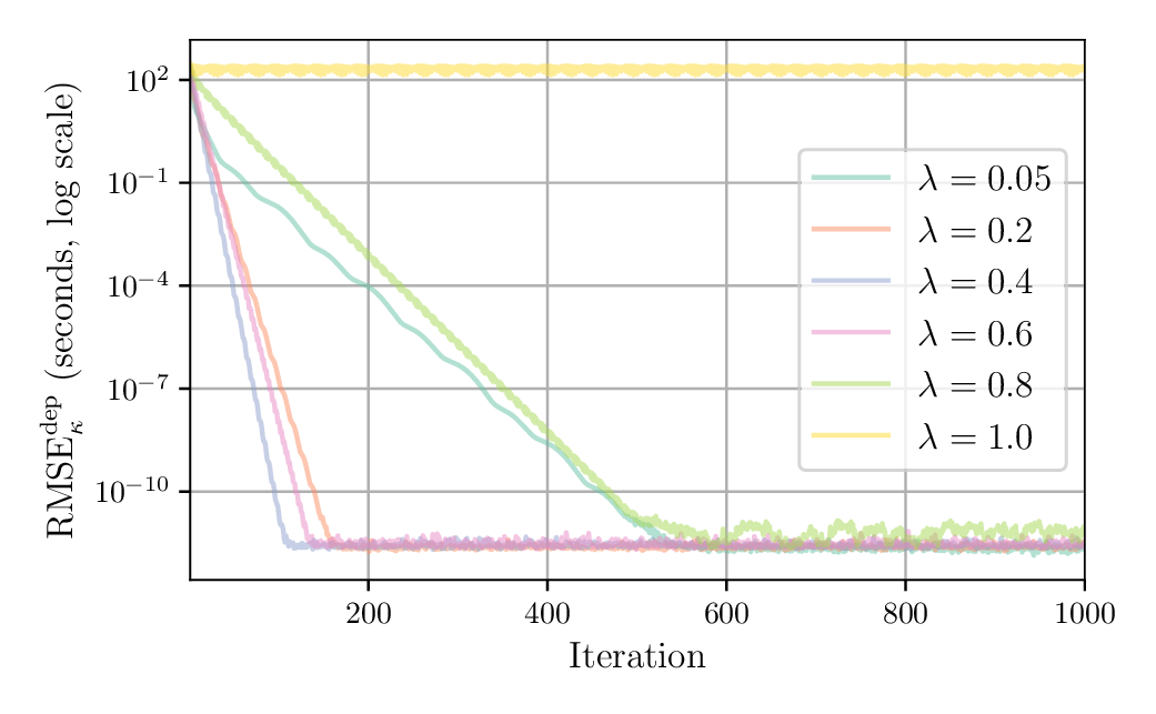
- For exponential smoothing method: With smaller $\lambda$, convergence is slower but steadier
Indicators: Road Network Conditions
exp_road_network_cond_rmse: Difference between the expected road-network conditions and the simulated road-network conditions-
Formula:
\[
\text{RMSE}_\kappa^{T} = \sqrt{\frac{1}{R} \sum_{r} \frac{1}{t^1 - t^0} \int_{t^0}^{t^1} [T_{r, \kappa}(t) - \hat{T}_{r, \kappa}(t)]^2 \text{d} t},
\]
- $T_{r, \kappa}(t)$: simulated travel time on link $r$, at time $t$, for iteration $\kappa$
- $\hat{T}_{r, \kappa}(t)$: expected travel time on link $r$, at time $t$, for iteration $\kappa$
- $R$: number of links
- $[t^0, t^1]$: simulation period
- Interpretation: Average difference in seconds between the expected and simulated travel times, over links and time
Indicators: Departure Time Shift
alt_dep_time_rmse: Difference between the departure times of the previous and current iteration-
Formula:
\[
\text{RMSE}_\kappa^{\text{dep}} = \sqrt{\frac{1}{N} \sum_n (t^{\text{d}}_{n, \kappa} - t^{\text{d}}_{n, \kappa-1})^2},
\]
- $t^{\text{d}}_{n, \kappa}$: departure time of agent $n$, at iteration $\kappa$
- $N$: number of agents
- Interpretation: By how much agents shifted their departure time from one iteration to another, only including the agents who did not switched to another alternative
Indicators: Travel Time Expectation Error
road_trip_exp_travel_time_diff_rmse: Difference between the expected travel time and the simulated travel time-
Formula:
\[
\text{RMSE}_\kappa^{\text{expect}} = \sqrt{ \frac{1}{K^{\text{road}}} \sum_{n, k} (tt_{n, k, \kappa} - \hat{tt}_{n, k, \kappa})^2 },
\]
- ${tt}_{n, k, \kappa}$: simulated travel time for trip $k$ of agent $n$, at iteration $\kappa$
- $\hat{tt}_{n, k, \kappa}$: expected travel time for trip $k$ of agent $n$, at iteration $\kappa$
- $K^{\text{road}}$: number of road trips
- Interpretation: By how much agents mis-predicted their travel time, for their road trips
- It measures both distance to an equilibrium and approximation errors due to the linear approximation of travel-time functions
Session 4 Task
Starting from you road network (Task of Session 2) and your population (Task of Session 3), create and run a complete simulation.
- Define the
parameters.jsonfile - Add alternatives with road trips to the population files
- Make sure that everything is compatible (origin / destination are valid road-network nodes, all routes are feasible, trips' vehicle ids are valid ids, etc.)
- Run!