METROPOLIS2 Course
Session 3: Demand Side
Lucas Javaudin
Spring 2024
Plan of this Session
- Introduction
- Mode Choice
- Road and Virtual Trips
- Departure-Time Choice
- Advanced Demand Modeling
- Task for Next Session
Sessions
- Introduction (13th March)
- Supply side: road network (27th March)
- Demand side: agents, travel alternatives and trips (3rd April)
- Technical parameters and running the simulator (10th April)
- Reading and understanding the results (17th April)
- Case-study: Paris' low-emission zone (Input)
- Case-study: Paris' low-emission zone (Output)
- Extensions: fuel consumption, CO2 emissions and local pollutants
METROPOLIS2 Fundamental Flow Diagram
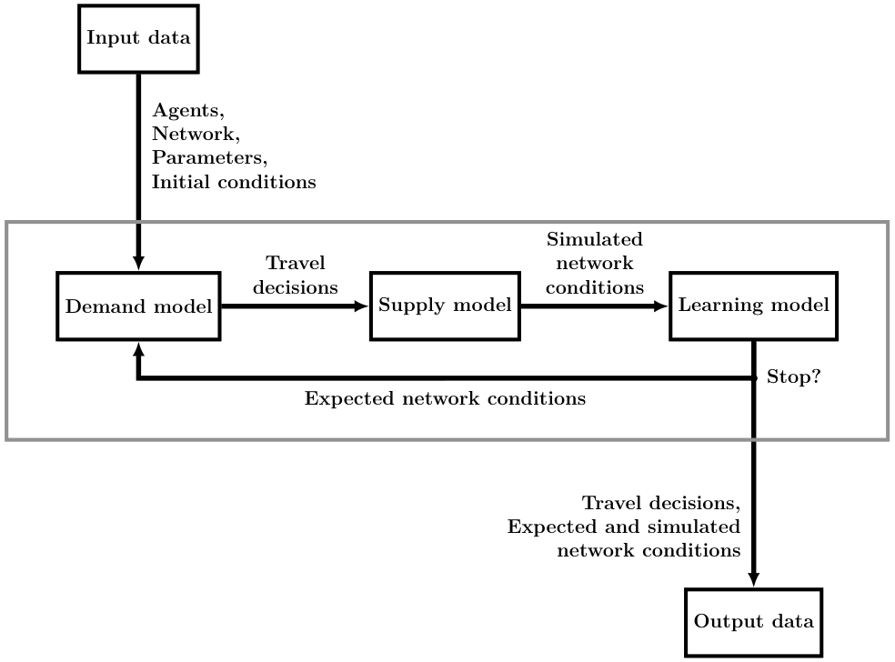
METROPOLIS2 Input Files
- Parameters (JSON)
-
Supply side:
- Road network (Parquet or CSV)
- Vehicle types (Parquet or CSV)
-
Demand side:
- Agents (Parquet or CSV)
- Travel alternatives (Parquet or CSV)
- Trips (Parquet or CSV)
- Optional road-network conditions (Parquet or CSV)
Documentation
For additional details and references on what is covered during this session, refer to the documentation
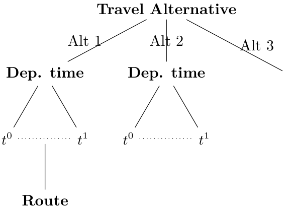
https://docs.metropolis.lucasjavaudin.com/getting_started/input/agents.htmlMETROPOLIS2 Decision Tree
- Level 1: choice between travel alternatives
- Level 2: choice of a departure time (except for no-trip alternatives)
- Level 3: choice of a route (for road trips only)
Parameters JSON File for this Session
To run the example simulations of this session, create the following
parameters.json file:
					{
						"input_files": {
							"agents": "agents.csv",
							"alternatives": "alts.csv"
						},
						"output_directory": "output",
						"max_iterations": 1,
						"period": [0.0, 3600.0],
						"saving_format": "CSV"
					}
Travel Alternatives
- Travel alternative: description of a plan / program / strategy that the agent can choose to execute
- Examples: travel from home to work by car; travel from home to work by public-transit then from work to shop by walking; do not travel
- All agents must have at least one alternative
- At each iteration, each agent is selecting exactly one alternative to execute
- In most cases, the choice of an alternative represents a mode choice
Run 1: No Mode Choice, No Utility
-
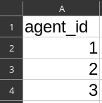
File
agents.csv:- Column
agent_id= 1,2,3
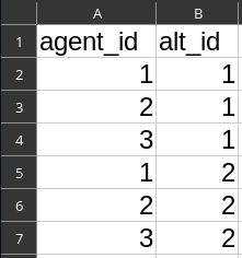
File
alts.csv- Column
agent_id= 1,2,3 - Column
alt_id= 1,1,1,2,2,2
- Column
- Run METROPOLIS2
-
Read the output file
agent_results.csv
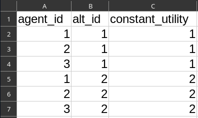
Run 2: Constant Utility
-
File
alts.csv- Column
constant_utility= 1,1,1,2,2,2
- Column
- Run METROPOLIS2
-
Read the output file
agent_results.csv When no mode choice (= alternative choice) is specified, the first alternative is always the chosen one.
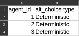
Run 3: Deterministic Mode Choice
-
File
agents.csv- Column
alt_choice.type= Deterministic
- Column
- Run METROPOLIS2
-
Read the output file
agent_results.csv All agents are choosing alternative 2 and get 2 utility units
Logit Model
- Consider an agent choosing between two alternatives 1 and 2
- (Deterministic) utility of alternative 1 (resp. 2) is $V_1$ (resp. $V_2$)
- Discrete-choice theory: total utility of alternative $j$ is \[ U_j = V_j + \varepsilon_j \]
- Logit model if $\varepsilon_j \overset{i.i.d.}{\sim} \textit{Gumbel}$
- Probability to choose alternative $1$ is \[ p_1 = \text{Prob}(U_1 > U_2) = \frac{e^{V_1}}{e^{V_1} + e^{V_2}} \]
- Expected utility from the choice \[ \mathbb{E}_{\varepsilon}[\max_j U_j] = \ln(e^{V_1} + e^{V_2}) + 0.577 \]
Multinomial Logit and Continuous Logit
Multinomial Logit
- Probability to choose alternative $j$: \[ p_j = \frac{e^{V_j / \mu}}{\sum_k e^{V_k / \mu}} \]
- Expected utility from the choice \[ \mathbb{E}_{\varepsilon}[\max_j U_j] = \mu \ln \sum_j e^{V_j / \mu} + \mu \cdot 0.577 \]
Continuous Logit
- Probability to choose interval $[t, t']$: \[ p([t, t']) = \frac{\int_{t}^{t'} e^{V(\tau) / \mu} \text{d} \tau}{\int_{t^0}^{t^1} e^{V(\tau) / \mu} \text{d} \tau} \]
- Expected utility from the choice \[ \mathbb{E}_{\varepsilon}[\max_\tau U(\tau)] = \mu \ln \int_{t^0}^{t^1} e^{V(\tau) / \mu} \text{d} \tau + \mu \cdot 0.577 \]
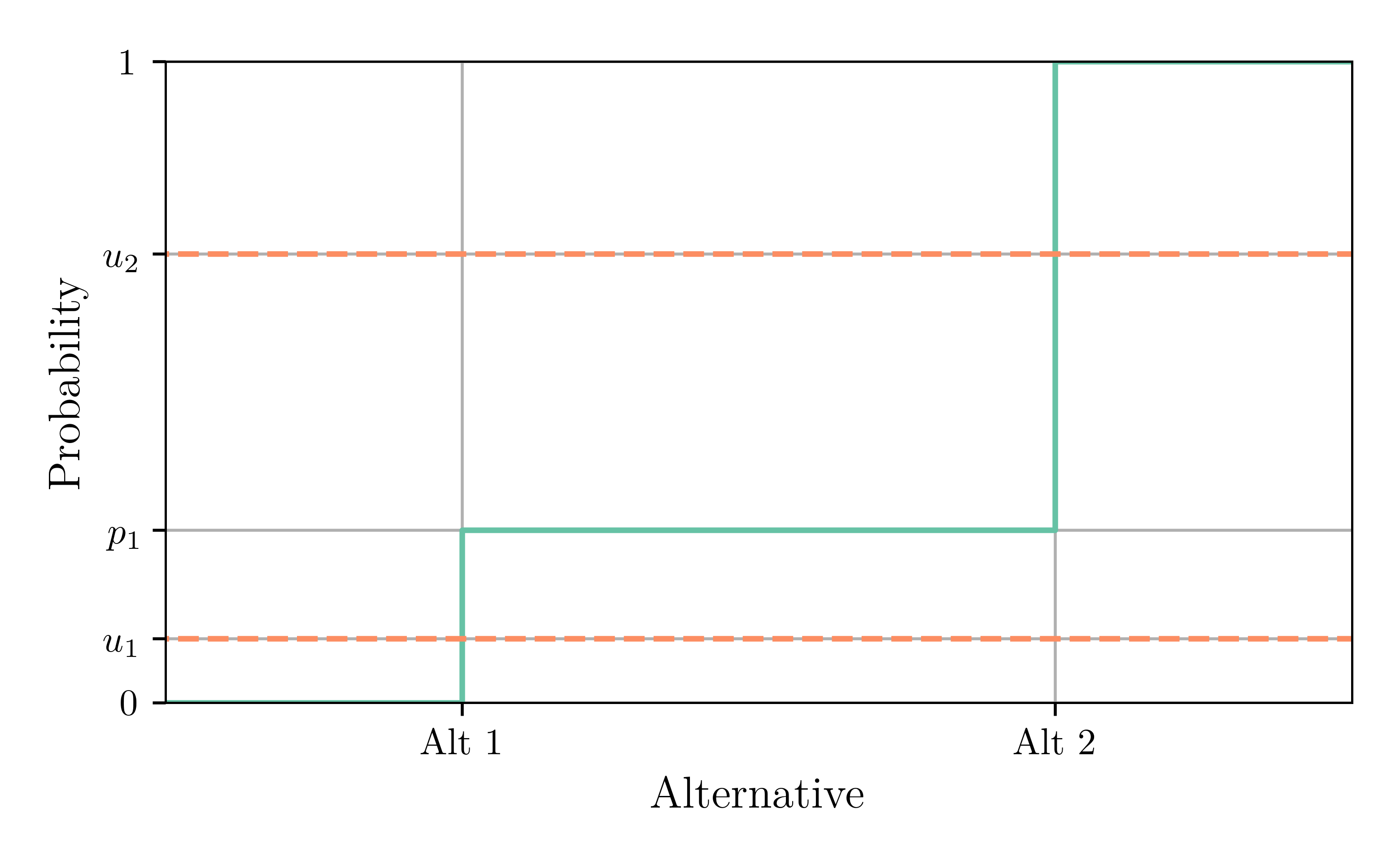
Inverse Transform Sampling
- Draw a value $u_n \sim \text{Uniform}([0, 1])$ for each agent
- Select alternative 1 if $u_n < p_1$
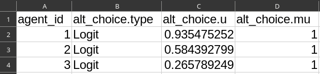
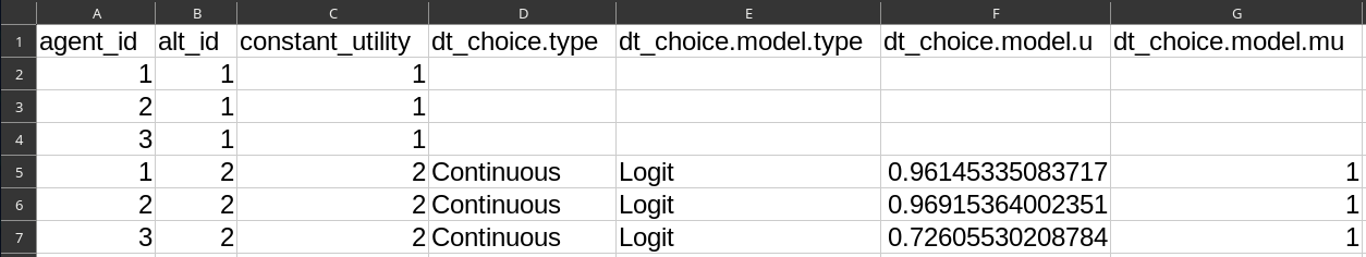
Run 4: Logit Mode Choice
-
File
agents.csv- Column
alt_choice.type= Logit - Column
alt_choice.u= RAND() - Column
alt_choice.mu= 1
- Column
- Run METROPOLIS2
-
Read the output file
agent_results.csv
Overview
- Each alternative consists in 0, 1 or more trip(s), to be executed sequentially
- Two types of trips: road and virtual
- Road trip: origin, destination, vehicle type (will be covered during Session 4)
- Virtual trip (or teleport trip): exogenous travel time (e.g., walking, cycling, public transit)
Parameters JSON File
Add the "trips.csv" file to the parameters
					{
						"input_files": {
							"agents": "agents.csv",
							"alternatives": "alts.csv",
							"trips": "trips.csv"
						},
						"output_directory": "output",
						"max_iterations": 1,
						"period": [0.0, 3600.0],
						"saving_format": "CSV"
					}
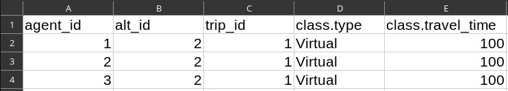
Run 5: Virtual Trip
-
File
alts.csv:- Column
dt_choice.type= Constant - Column
dt_choice.departure_time= 50
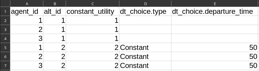
File
trips.csv:- Column
agent_id= 1,2,3 - Column
alt_id= 2,2,2 - Column
trip_id= 1,1,1 - Column
class.type= Virtual - Column
class.travel_time= 100
- Column
- Run METROPOLIS2
-
Read the output file
agent_results.csv
Travel Utility
-
Utility of a no-trip alternative is simply equal to
constant_utility - Utility of an alternative with a single trip is equal to \[ \text{utility} = \texttt{constant\_utility} + \texttt{travel\_utility.one} \times \text{travel\_time} \]
- Variables
travel_utility.two,travel_utility.threeandtravel_utility.fourcan be use for a polynom of up to degree 4 - Schedule-delay utility can also be added (to be seen in the next part)
Run 6: Travel Utility
-
File
trips.csv:- Column
travel_utility.one= -0.01,-0.01,-0.01
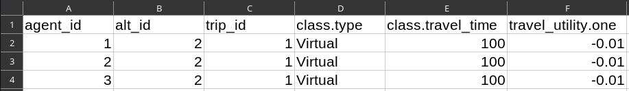
- Column
- Run METROPOLIS2
-
Read the output file
agent_results.csv Read the output file
trip_results.csv
Trip Chaining
- Each alternative can contain an arbitrary number of trips (a mix of road and virtual trips is possible)
- The trips are performed in the order in which they appear in the trips input file
- The
stopping_timevariable can be used to add a delay between two trips (this can represent the activity duration)
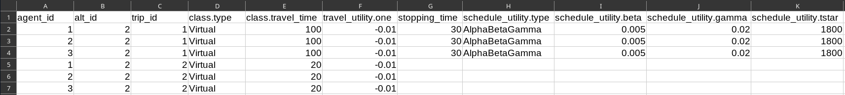
Run 7: Trip Chaining
-
File
trips.csv:- Column
agent_id= 1,2,3,1,2,3 - Column
alt_id= 2,2,2,2,2,2 - Column
trip_id= 1,1,1,2,2,2 - Column
class.type= Virtual
- Column
class.travel_time= 100,100,100,20,20,20 - Column
travel_utility.one= -0.01 - Column
stopping_time= 30,30,30,,,
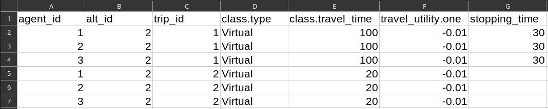
- Column
- Run METROPOLIS2
-
Read the output files
agent_results.csvandtrip_results.csv

Overview
- Three types of departure-time approaches: Constant (dynamic traffic assignment), Continuous choice (Continuous Logit model), Discrete choice
- The only decision variable for departure-time choice is the departure time for the first trip of the trip chain → the departure time for the subsequent trips depends of the previous' trips travel times and stopping times
- The departure-time choice is based on the (anticipated) utility for the entire trip chain
Continuous Logit
- Probability to choose interval $[t, t']$: \[ p([t, t']) = \frac{\int_{t}^{t'} e^{V(\tau) / \mu} \text{d} \tau}{\int_{t^0}^{t^1} e^{V(\tau) / \mu} \text{d} \tau} \]
- Expected utility from the choice \[ \mathbb{E}_{\varepsilon}[\max_\tau U(\tau)] = \mu \ln \int_{t^0}^{t^1} e^{V(\tau) / \mu} \text{d} \tau + \mu \cdot 0.577 \]
With a constant utility function ($V(\tau) = \bar{V}$):
- Probability to choose interval $[t, t']$: \[ p([t, t']) = \frac{t' - t}{t^1 - t^0} \]
- Expected utility from the choice \[ \mathbb{E}_{\varepsilon}[\max_\tau U(\tau)] = \bar{V} + \mu \cdot \ln(t^1 - t^0) + \mu \cdot 0.577 \]
Run 8: Continuous Departure-Time Choice
-
File
alts.csv:- Column
dt_choice.type= Continuous - Column
dt_choice.model.type= Logit - Column
dt_choice.model.u= RAND() - Column
dt_choice.model.mu= 1
- Column
- Run METROPOLIS2
-
Read the output files
agent_results.csv
Expected Utility vs Alt Expected Utility vs Utility
-
utility: Simulated utility, based on the selected alternative $j$ and departure time $\tau$: $V^{\text{sim}}_{j}(\tau)$ -
alt_expected_utility: Expected utility of the departure-time choice of the selected alternative $j$: $\mathbb{E}_{\varepsilon}[\max_{\tau} U_j(\tau)]$ -
expected_utility: Expected utility of the alternative choice: $\mathbb{E}_{\varepsilon}[\max_{j} U_j]$
Utility
- Utility of a trip is \[ \text{trip utility} = \text{travel utility} + \text{schedule utility} \] with \[ \text{travel utility} = \texttt{travel\_utility.one} \times {tt} \] and \[ \text{schedule utility} = -\texttt{beta} \times [\texttt{tstar} - t^a]_+ - \texttt{gamma} \times [t^a - \texttt{tstar}]_+ \]
- Total utility of a travel alternative is \[ \text{utility} = \texttt{constant\_utility} + \sum_{\text{trip}} \text{trip utility} \]
Run 9: Schedule-Delay Utility
-
File
trips.csv:- Column
schedule_utility.type= AlphaBetaGamma - Column
schedule_utility.tstar= 1800 - Column
schedule_utility.beta= 0.005 - Column
schedule_utility.gamma= 0.02
- Column
- Run METROPOLIS2
-
Read the output file
trip_results.csv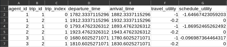
Alternative Choice
- At the top level, agents choose among an arbitrary number of travel alternatives
- A travel alternative is defined as a sequence of trips and a utility function specification
-
The alternative choice can represent:
- Mode choice: H→W by car | H→W by PT | H→W by walk
- Mode choice with trip chaining: H→W→S→H by car | H→W→S→H by bicycle
- To travel or not to travel: H→W by car | No trip (work-from-home)
- Inter-modality: H→P by car then P→W by PT | H→W by car
- Destination choice: H→S1 by walk | H→S2 by walk
- Vehicle choice: H→W with a fast but energy-consuming car | H→W with a fuel-efficient but slow car
Choice Models
- Alternative choice: Multinomial Logit or Deterministic
- Departure-time choice: Continuous Logit or Multinomial Logit
- Almost any discrete-choice model is feasible by drawing the epsilon values (idiosyncratic chocs) "offline" and specifying them in the utility
- Selecting alternative $A$ with probability $p = e^{V_a} / (e^{V_a} + e^{V_b})$ using inverse transform sampling is equivalent to selecting alternative $A$ if and only if $V_A + \varepsilon_A > V_B + \varepsilon_B$ where $\varepsilon_A$ and $\varepsilon_B$ are two Gumbel-distributed values
- Example for a Probit mode choice with three alternatives:
- Draw $\varepsilon_j \sim \mathcal{N}(0, 1), j \in \{1, 2, 3\}$
- Add $\varepsilon_j$ to the utility of alternative $j$ in the simulator
- Select a deterministic choice model (the value maximizing $V_j + \varepsilon_j$ is selected)
Input data
Two main ways to generate population data:
- Origin-Destination Matrix: For any row $i$ and colomun $j$ in the matrix, generate $a_{ij}$ agents with a single trip from origin $i$ to destination $j$
-
Synthetic Population:
- Given various data (census, travel survey, etc.), the synthetic population algorithm returns a list of agents and the activities they perform
- Easily convertible to METROPOLIS2 input format
- Travel times for virtual trips can be computed using METROPOLIS2's routing algorithm (See Session 2)
- Example for France: Hörl, S. and M. Balac (2021) Synthetic population and travel demand for Paris and Île-de-France based on open and publicly available data, Transportation Research Part C
Session 3 Task
Create your own population of agents using various features presented in this session (alternative choice, no-trip alternatives, virtual trips, trip chaining, schedule utility, departure-time choice, etc.)