METROPOLIS2 Course
Session 2: Supply Side
Lucas Javaudin
Spring 2024
Plan of this Session
- Getting Started with METROPOLIS2 (cont.)
- Congestion Modeling in METROPOLIS2
- Edges Input File
- Vehicle Types Input File
- Road-Network Parameters
- Routing
- OpenStreetMap Import
- Task for Next Session
The METROPOLIS2 Website
https://metropolis.lucasjavaudin.comRunning METROPOLIS2 (the Easy Way, on Windows)
- Download the last GUI version of METROPOLIS2 for Windows (tab Download on the website).
- Execute the .msi file and follow the procedure to install METROPOLIS2 (accept the non-existent risks if the antivirus complains).
- Run the METROPOLIS2 program that is now installed on your computer.
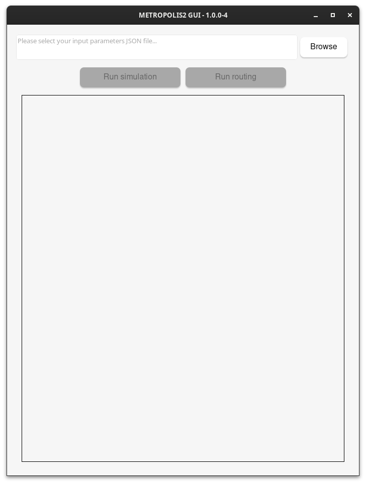
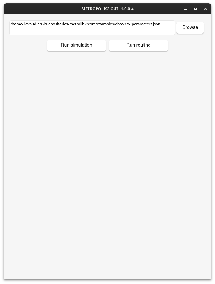
- Click on
Browseand select yourparameters.jsonfile. - Click on the
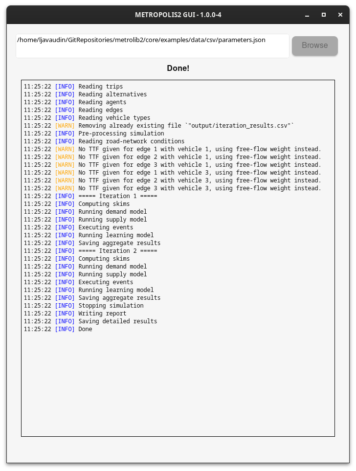
Run simulationbutton. - Check the logs and close the window when you are done.
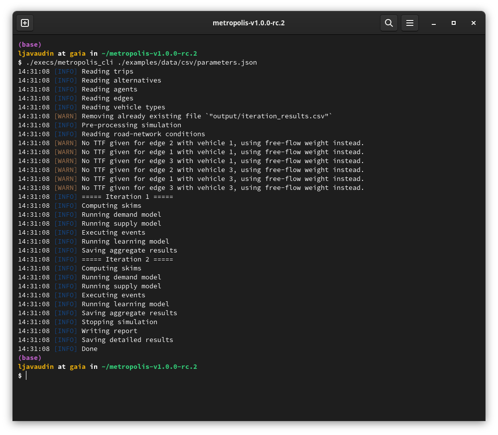
Running METROPOLIS2 (the Hard Way)
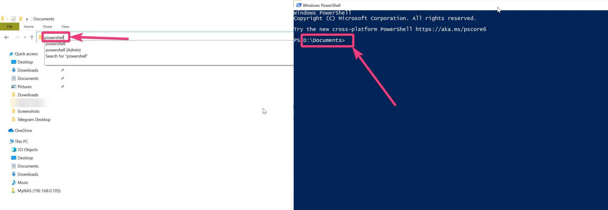
- Open a Command prompt / Terminal / Powershell with the working directory set to the location of the unzipped directory
-
For Windows, run:
.\execs\metropolis_cli.exe .\examples\data\csv\parameters.json -
For MacOS or Linux, run:
./execs/metropolis_cli ./examples/data/csv/parameters.json - Check that the run succeeded
- The results are stored in
examples/data/csv/output/
METROPOLIS2 Input Files
- Parameters (JSON)
-
Supply side:
- Road network (Parquet or CSV)
- Vehicle types (Parquet or CSV)
-
Demand side:
- Agents (Parquet or CSV)
- Travel alternatives (Parquet or CSV)
- Trips (Parquet or CSV)
- Optional road-network conditions (Parquet or CSV)
METROPOLIS2 Output Files
- HTML summary
- Aggregated results by iteration (Parquet or CSV)
-
Supply side:
- Link-level time-dependent travel times (simulated, expected for last iteration and expected for next iteration) (Parquet or CSV)
- OD-level time-dependent travel times (expected for last iteration) (JSON, for now)
-
Demand side:
- Agent-level results (Parquet or CSV)
- Trip-level results (Parquet or CSV)
- Routes taken (Parquet or CSV)
Files Format: JSON
-
Collection of key-value pairs that can be nested indefinitely
{ "key": "value", "myint": 1, "myfloat": 3.6, "mybool": true, "myarray": [ 0, 1, 2 ], "nested_array": [ { "some": "value", "another": "value" }, {"second": "object"} ] } - Very close to Python's
dicttype - Format used to configure the parameters of a METROPOLIS2 simulation and for some output files
- Syntax definition: https://en.wikipedia.org/wiki/JSON#Syntax
Files Format: CSV
- Row-oriented file format for tabular data
- Human readable
- Compatible with many tools and languages (including Excel!)
- Used in METROPOLIS2 for most input and output files (comma separator only)
- Recommended only for small-scale simulations, especially when using Excel
Example of CSV file:
						col1,col2,col3,col4
						1,Alice,3.2,true
						2,Bob,1.4,false
						3,Charlie,2.5,false
Files Format: Parquet
- Column-oriented file format for tabular data
- Binary file (= non human-readable)
- Built-in compression: smaller file size than CSV
- Very fast
- Compatible with Python (polars or pandas libraries) and R (arrow package)
- Used in METROPOLIS2 for most input and output files
- Recommended format for large-scale simulations and people working with R or Python
						import polars as pl

						df = pl.DataFrame(
								{
										"agent_id": [0, 1, 2],
										"alt_choice.type": ["Deterministic", "Logit", "Logit"],
										"alt_choice.u": [0.3, 0.6, 0.5],
										"alt_choice.mu": [None, 0.9, 1.0],
										"alt_choice.constants": [[0.9, 1.3, 2.1], None, None],
								}
						)
						df.write_parquet("input/agents.parquet")
						In [3]: df
						Out[3]:
						shape: (3, 5)
						┌──────────┬─────────────────┬──────────────┬───────────────┬──────────────────────┐
						│ agent_id ┆ alt_choice.type ┆ alt_choice.u ┆ alt_choice.mu ┆ alt_choice.constants │
						│ ---      ┆ ---             ┆ ---          ┆ ---           ┆ ---                  │
						│ i64      ┆ str             ┆ f64          ┆ f64           ┆ list[f64]            │
						╞══════════╪═════════════════╪══════════════╪═══════════════╪══════════════════════╡
						│ 0        ┆ Deterministic   ┆ 0.3          ┆ null          ┆ [0.9, 1.3, 2.1]      │
						│ 1        ┆ Logit           ┆ 0.6          ┆ 0.9           ┆ null                 │
						│ 2        ┆ Logit           ┆ 0.5          ┆ 1.0           ┆ null                 │
						└──────────┴─────────────────┴──────────────┴───────────────┴──────────────────────┘
Units
For consistency and to prevent mistakes, METROPOLIS2 uses the same units for all input and output variables.
| Type | Unit | Example |
|---|---|---|
| Time duration | Seconds | 300 (5 minutes) |
| Time of day | Seconds after midnight | 8 * 3600 = 28800 is 8 a.m. |
| Length | Meters | |
| Speed | Meters / Second | 50 / 3.6 = 13.89 m/s is 50 km/h |
| Passenger Car Equivalent (PCE) | N/A | Usually normalized to 1 for car |
| Flow | PCE / Second | 0.5 PCE/s = 1800 PCE per hour |
| Utility | No specific unit (can be monetary units) | |
| Value of Time | Utility / Second | 15 / 3600 = 0.004167 is 15 $/h |
Mistakes are still possibles, be careful!
Sources of Congestion
METROPOLIS2 is a mesoscopic simulator with three sources of congestion:
- Bottleneck: the inflow and outflow of vehicles is limited at the link-level
- Speed-density function: the speed of vehicles depends on the density of vehicles currently on the link
- Queue propagation (or spillback, or horizontal queues): vehicles can enter a link only if there is some space available
Users can choose to enable only some sources of congestion.
There is no en-route choice in METROPOLIS2
Vehicle Types
METROPOLIS2 can simulate vehicle types with different:
- Headway length (head-to-head) → for speed-density functions and spillback evaluation
- PCE (Passenger Car Equivalent) → for bottlenecks
- Speed functions → e.g., to represent speed limits
- Road restrictions → allowed / forbidden links
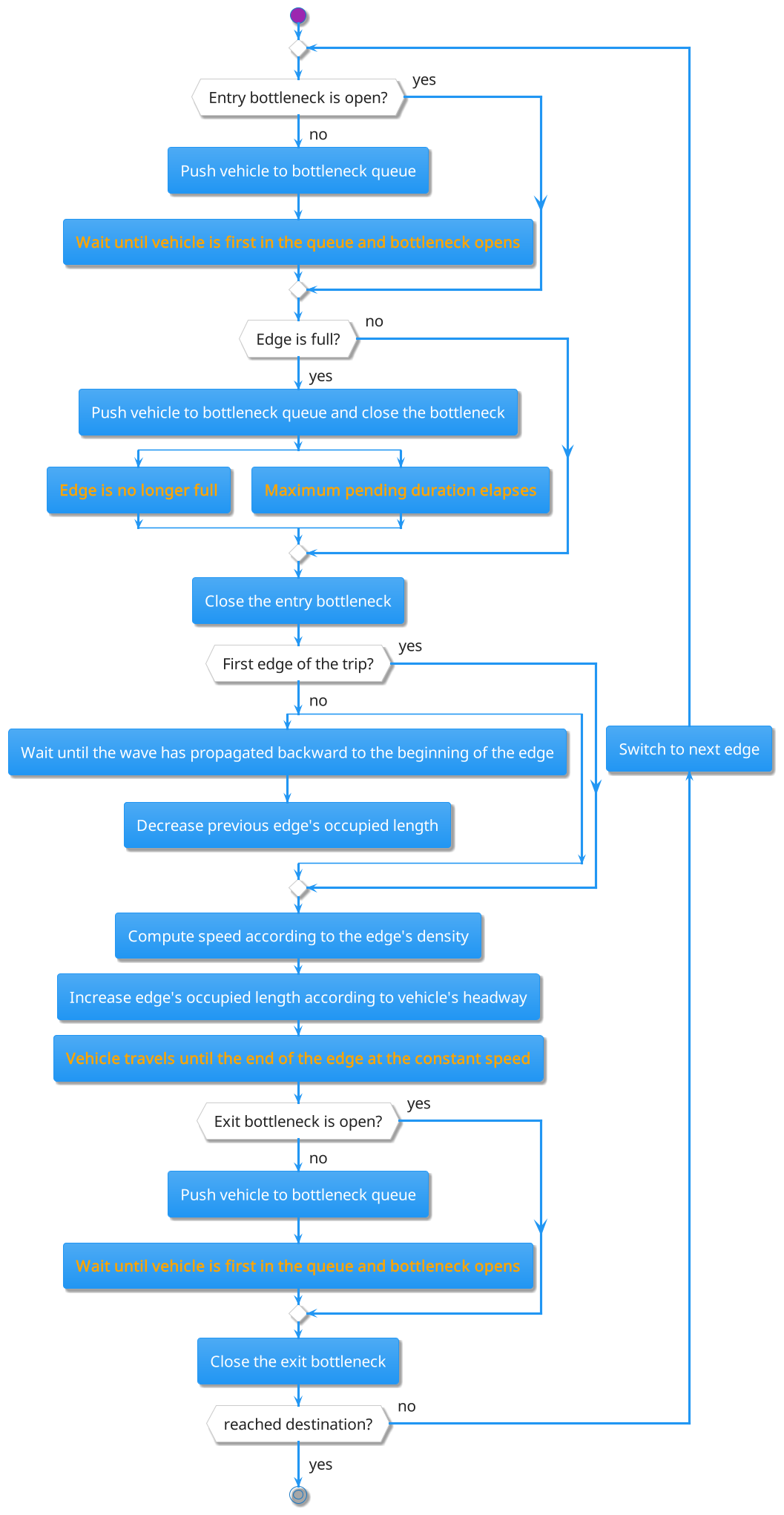
Simplified Process
How vehicles travel through a link in METROPOLIS2?
- Cross the entry bottleneck if it is open, or wait until it opens
- Enter the link if there is some space available, or wait for some space to be available again
- Travel across the length of the link at a constant speed given based on the density of vehicles on the link at the entry time
- Cross the exit bottleneck if it is open, or wait until it opens
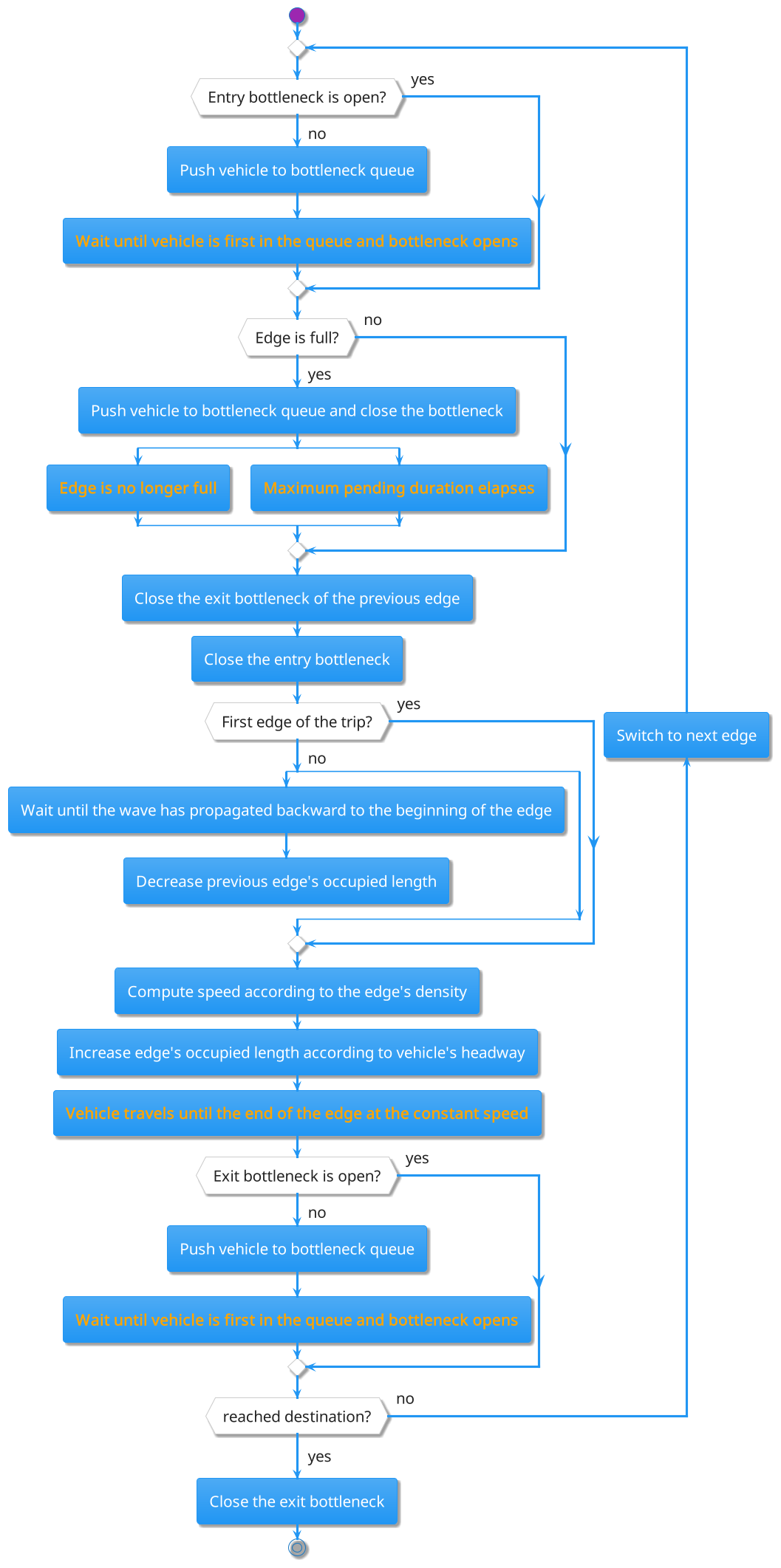
Full Process
Bottleneck
- One bottleneck at the entry and exit of each link
- Bottlenecks can be in two states: open or closed
- Bottlenecks are open by default and open bottlenecks can be crossed immediately
- When a vehicle cross a bottleneck, the bottleneck gets closed for a duration \[ \text{closing time} = \frac{\text{Vehicle PCE}}{\text{Bottleneck flow}} \]
- When a vehicle reaches a closed bottleneck, it is pushed to the back of the bottleneck queue
- When a closed bottleneck re-opens, the vehicle at the front of the queue can cross
- Question: bottleneck flow of 1200 PCE/h; a truck (3 PCEs) is crossing it; what is the closing time?
- Answer: 3 / (1/3) = 9
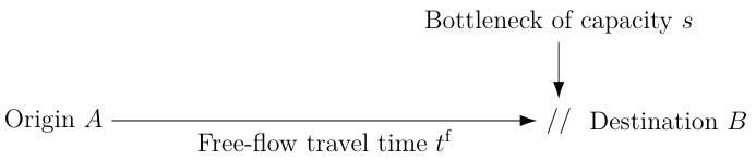
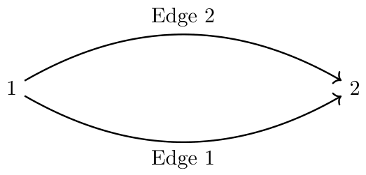
Bottleneck: Two Roads
-
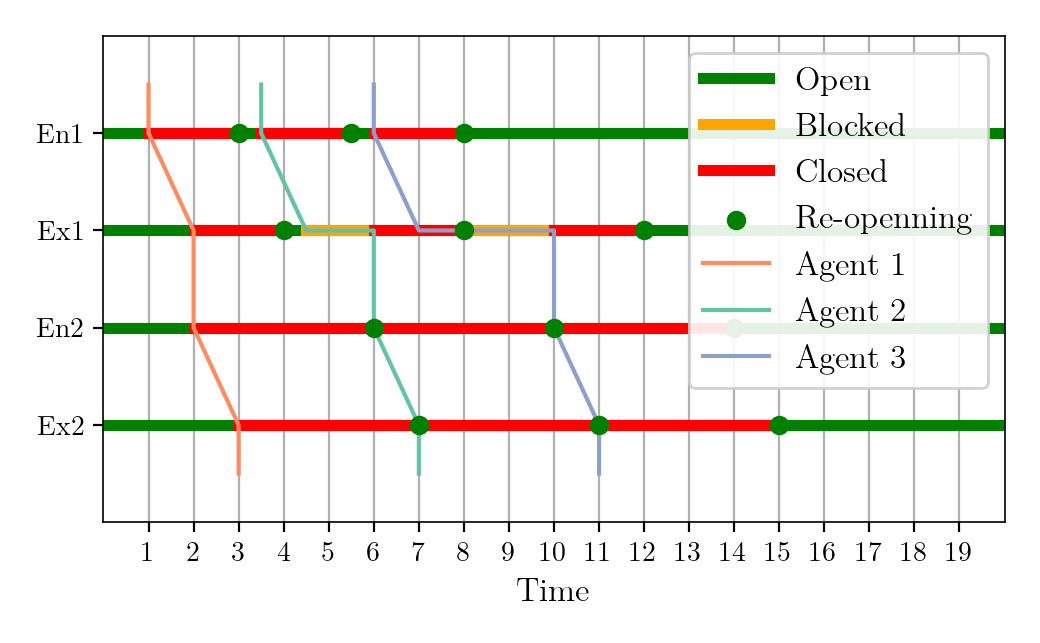
Example: Two successive roads with 1 second free-flow travel time and bottleneck flow of 0.5 and 0.25 PCE/s (closing time of 2s and 4s for 1 PCE).

- Consider agents traveling from 1 to 3 with departure times [1, 3.5, 6]. What are the arrival times?
- Agent 1: enters edge 2 at time 2; arrives at time 3.
- Agent 2: reaches edge 2 at time 4.5; enters edge 2 at time 6; arrives at time 7.
- Agent 3: reaches edge 2 at time 7; enters edge 2 at time 10; arrives at time 11.
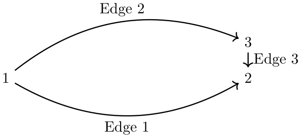
Bottleneck: Two Roads
- Departure times [1, 3.5, 6]
- Arrival times [3, 7, 11]
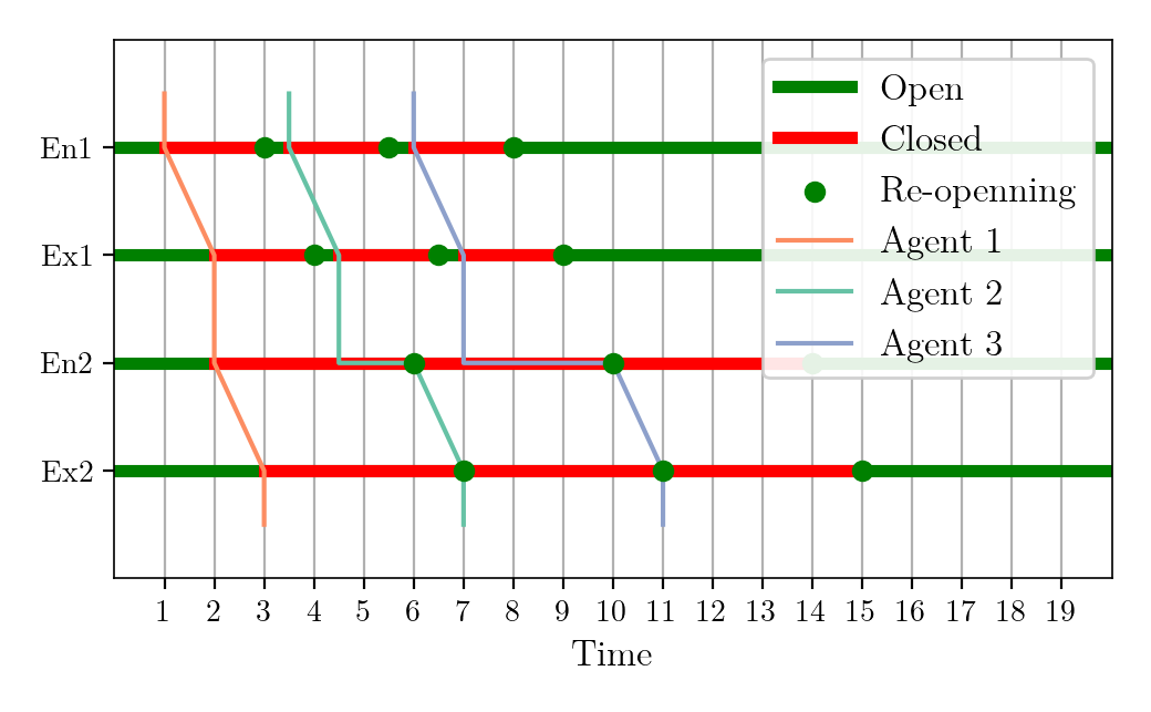
Where exactly is Agent 3 from time 7 to time 10?
Overtaking
- When traveling to the end of the link, faster moving vehicles can overtake slower vehicles
- By default, when a vehicle is stuck at the entry of a link (entry bottleneck closed or no space available), the exit bottleneck of the previous link stays closed → vehicles upstream are also stuck
- If enabled, the exit bottleneck of the previous link re-opens as soon as a vehicle cross (even if it is stuck downstream) → vehicles upstream can overtake the vehicle if they are going to different downstream links
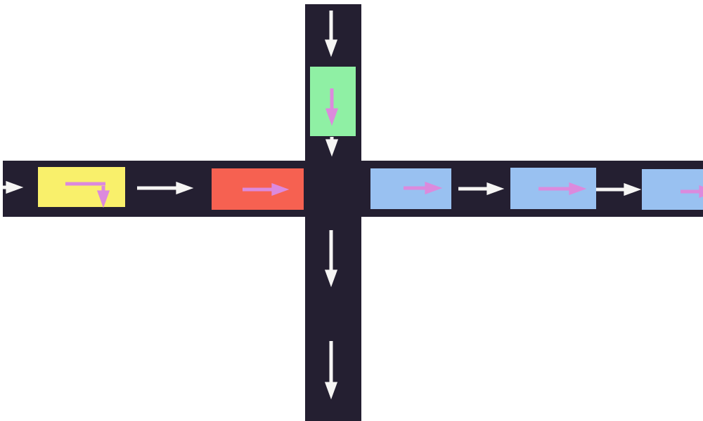
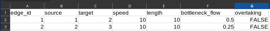
Bottleneck Overtaking: Two Roads
Overtaking = TRUE
Overtaking = FALSE
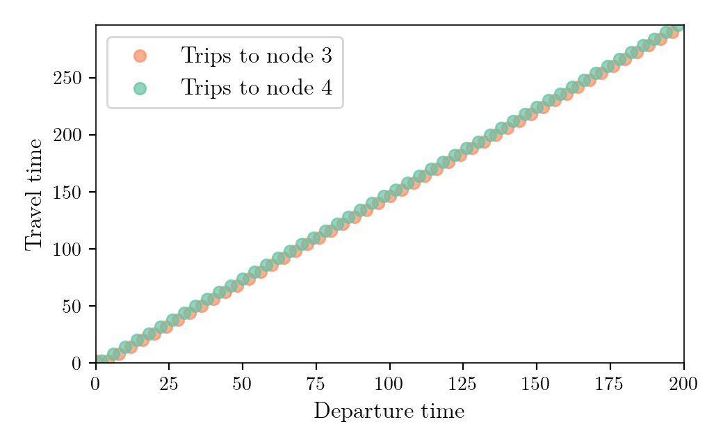
Bottleneck Overtaking: Three Roads
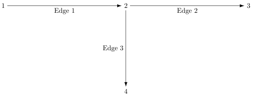
- Each 2 seconds, a car is starting from node 1.
- One out of two cars is going to node 3, the other is going to node 4.
- Bottleneck capacity is large for edges 1 and 2 but small for edge 3.
Bottleneck Overtaking: Three Roads
Overtaking = TRUE
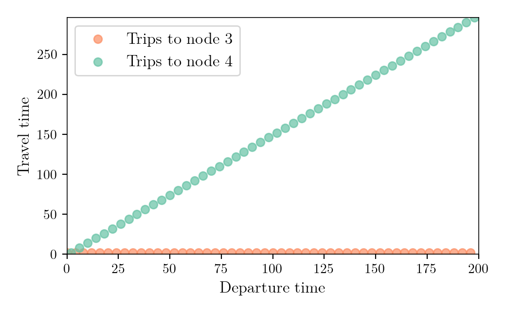
Overtaking = FALSE
Number of Lanes
The number of lanes on a link has only two impacts:
- The bottleneck flow of a link is multiplied by the number of lanes
- The space available on the link is multiplied by the number of lanes (relevant for spillback only)
Speed-Density Functions
- The speed at which a vehicle travel over the length of an edge is constant and computed using the edge's speed-density function
- The speed-density returns the traveling speed on the edge as a function of the current density of vehicles on the edge
- The edge's density is computed as \[ \text{density} = \frac{\sum_{\text{vehicle on the edge}}\text{headway length of vehicle}}{\text{length} \times \text{lanes}} \]
- Three speed-density functions: FreeFlow (default), Bottleneck (METROPOLIS1 legacy), ThreeRegimes
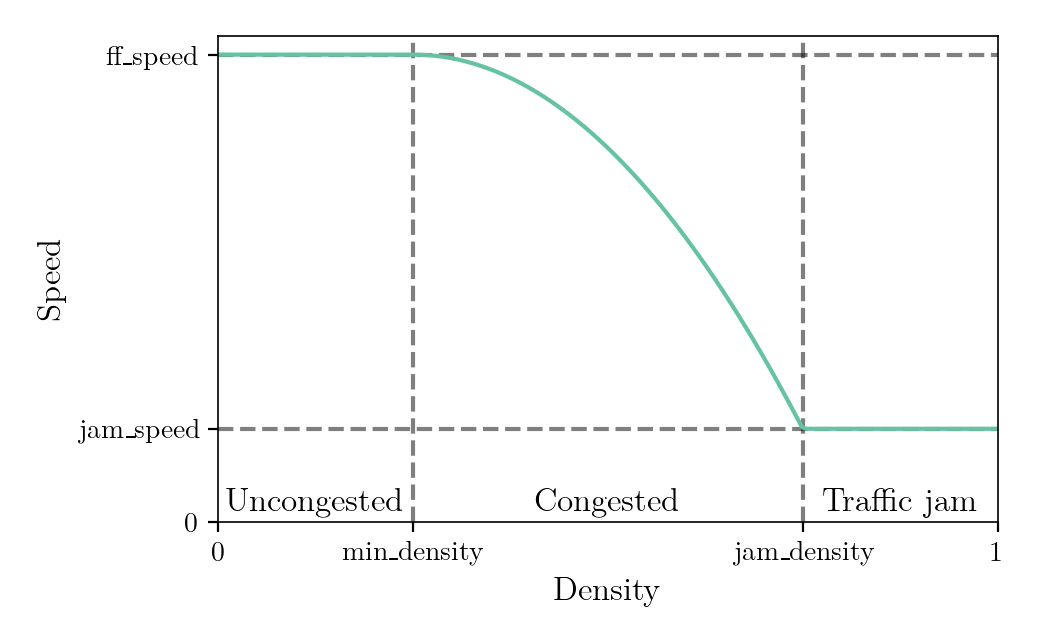
Speed-Density Functions: Three Regimes
\[
\text{speed}(\text{density}) =
\left\{\begin{array}{ll}
\text{ff\_speed} & \text{if density} < \text{min\_density} \\
\text{jam\_speed} & \text{if density} > \text{jam\_density} \\
\text{ff\_speed} \times (1 - \alpha) + \text{jam\_speed} \times \alpha & \text{otherwise} \\
\end{array}\right.
\]
\[
\alpha = \left( \frac{\text{density} - \text{min\_density}}{\text{jam\_density} - \text{min\_density}} \right)^\beta
\]
\(\beta = 1\): linear; \(\beta < 1\): convex; \(\beta > 1\): concave
Spillback
- If spillback is enabled, vehicles can enter an edge only if there some room left on the edge ($\Leftrightarrow$ density < 1)
- If the edge ahead is full, the vehicle is remaining in the exit bottleneck queue of the current edge, in a "pending state"
- When a vehicle exits an edge, the space taken by this vehicle propagates backward at a given speed (backward wave propagation)
- Time at which the space of an outgoing vehicle is made available for the incoming vehicles: \[ \text{exit\_time} + \frac{\text{length}}{\text{backward\_wave\_speed}} \]
Gridlocks
- When spillback is enabled, the road network can reach a state where some vehicles are permanently stuck
- The maximum pending duration defines the maximum amount of time a vehicle can be in a pending state
- After the maximum pending duration elapses, pending vehicles are forced onto the next edge
Full Process
Overtaking = TRUE
Overtaking = FALSE
Overview
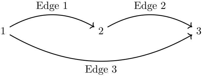
- The simulator represents the road network as a directed graph of nodes (= intersections) and edges (= links)
- METROPOLIS2 takes as input a list of edges
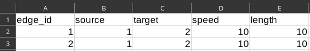
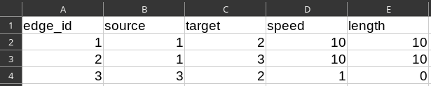
Minimal Example
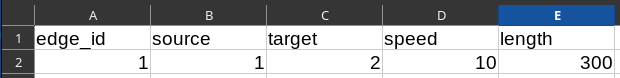
edge_id: Identifier of the edge (positive integer, unique)source: Identifier of the source node (positive integer)target: Identifier of the target node (positive integer)speed: Free-flow speed on the edge (m/s)length: Length of the edge (m)
Bottleneck

bottleneck_flow: Maximum inflow and outflow of the edge (PCE/s)- When the variable is omitted, the inflow and outflow are not limited
Bottleneck Overtaking
overtaking: If `True`, vehicles can overtake other vehicles in the bottleneck queues if they are going to different edges- Default value is `True`
Number of Lanes

lanes: number of lanes available to vehicles on the edge (in the current direction)- If omitted, the number of lanes is set to 1
- Non-integer values can be used
Speed-Density Functions

- With
speed_density.type = "FreeFlow"(or when omitting the variable, the speed on the link is always equal to the free-flow speed - With
speed_density.type = "ThreeRegimes", the "Three Regimes" speed-density function is used and the following parameters need to be set:speed_density.min_density,speed_density.jam_density,speed_density.jam_speedandspeed_density.beta
\[
\text{speed}(\text{density}) =
\left\{\begin{array}{ll}
\text{ff\_speed} & \text{if density} < \text{min\_density} \\
\text{jam\_speed} & \text{if density} > \text{jam\_density} \\
\text{ff\_speed} \times (1 - \alpha) + \text{jam\_speed} \times \alpha & \text{otherwise} \\
\end{array}\right.
\]
\[
\alpha = \left( \frac{\text{density} - \text{min\_density}}{\text{jam\_density} - \text{min\_density}} \right)^\beta
\]
Travel Time Penalty

constant_travel_time: time penalty that is added to the edge's travel time, in seconds- Travel-time on the edge is (excluding the waiting times): \[ \text{constant\_travel\_time} + \frac{\text{length}}{\text{speed}(\text{density})} \]
- This penalty can represent delays which happen even under free-flow conditions (e.g., waiting at traffic lights, stopping at a stop sign)
- The default value is zero
Parallel Edges
-
The METROPOLIS2 Routing algorithm cannot handle edges with the same source and target (parallel edges)
-
Possible workaround if required:
Documentation
For additional details, go to the documentation
https://docs.metropolis.lucasjavaudin.com/getting_started/input/road-network.htmlMinimal Example
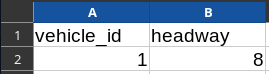
vehicle_id: Identifier of the vehicle (positive integer, unique)headway: Head-to-head length between two vehicles (m, used to compute edge's density)
Passenger-Car Equivalent
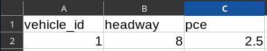
pce: Passenger-car equivalent for the vehicle (non-negative number)- Used to compute the closing time of bottlenecks
- Default value is 1
Speed Function
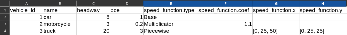
- The "Multiplicator" speed function type can be used to increase / decrease the speed of vehicles by a multiplicative coefficient
-
The "Piecewise" speed function type can be used to specify speed limits (e.g., vehicles limited to 90 km/h)
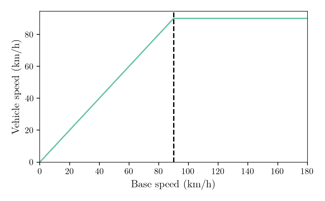
- Warning: lists are only supported for the Parquet format so the "Piecewise" type does not work for CSV
Road Restrictions

- Cars are allowed on all edges
- Motorcycles are only allowed on edges 1 and 2
- Trucks are allowed on all edges but edges 3 and 4
- Warning: lists are only supported for the Parquet format so the road restrictions do not work for CSV
Parameters JSON Input File
- The parameters JSON input file contains configuration values for the simulation (e.g., path to the input files, simulated period, learning model)
- A part of the file is dedicated to road-network parameters
- The remaining parts will be covered during the next sessions
							{
								[...]
								"road_network": {
									"recording_interval": 300.0,
									"approximation_bound": 1.0,
									"spillback": true,
									"backward_wave_speed": 4.0,
									"max_pending_duration": 60.0,
									"constrain_inflow": true,
									"algorithm_type": "Best",
								},
								[...]
							}
Travel-Time Function Parameters
recording_interval: time, in seconds, between two breakpoints in the edge-level travel-time functions (Mandatory; Recommendation: 5, 10 or 15 minutes for large-scale networks)approximation_bound: for a given travel-time function, if the difference between the maximum and the minimum travel time is smaller than this value, the function is represented as a constant function for optimization (Default: 0; Recommendation: between 0 and 5 seconds)
							{
								[...]
								"road_network": {
									"recording_interval": 300.0,
									"approximation_bound": 1.0,
									"spillback": true,
									"backward_wave_speed": 4.0,
									"max_pending_duration": 60.0,
									"constrain_inflow": true,
									"algorithm_type": "Best",
								},
								[...]
							}
Spillback Parameters
spillback: whether spillback congestion (queue propagation) is enabled (Default: TRUE; Recommendation: TRUE for more realistic congestion modeling)backward_wave_speed: speed at which the space taken by vehicles propagates backward upon exit (Default: instantaneous propagation; Recommendation: default or 15 km/h = 4.17 m/s)max_pending_duration: maximum amount of time a vehicle can stay in a pending state (Mandatory; Recommendation: between 30s and 5m, larger values are more realistic but generate more congestion)
							{
								[...]
								"road_network": {
									"recording_interval": 300.0,
									"approximation_bound": 1.0,
									"spillback": true,
									"backward_wave_speed": 4.0,
									"max_pending_duration": 60.0,
									"constrain_inflow": true,
									"algorithm_type": "Best",
								},
								[...]
							}
Other Parameters
constrain_inflow: whether bottlenecks limit vehicle inflow in addition to vehicle outflow (Default: TRUE; Recommendation: TRUE, set to FALSE to replicate MATSim behavior)algorithm_type: routing algorithm to use for profile queries, "Best", "TCH", or "Intersect" (Default: "Best"; Recommendation: "Intersect" for a smaller running time, "TCH" for a smaller memory consumption)
							{
								[...]
								"road_network": {
									"recording_interval": 300.0,
									"approximation_bound": 1.0,
									"spillback": true,
									"backward_wave_speed": 4.0,
									"max_pending_duration": 60.0,
									"constrain_inflow": true,
									"algorithm_type": "Best",
								},
								[...]
							}
Overview
- METROPOLIS2 relies on time-dependent Contraction Hierarchies algorithms
- Pre-processing phase: nodes are "contracted" from least "important" to most "important"; contracting a node entail removing it and the adjacent edges, while creating shortcut edges to maintain fastest paths
-
Two types of queries:
- Earliest-arrival query: Retrieve the earliest arrival time (= the minimum travel time) and the corresponding path, for a given origin-destination pair and departure time from origin
- Profile query: Retrieve the travel-time function, for a given origin-destination pair (minimum travel time for all possible departure times)
Query Types
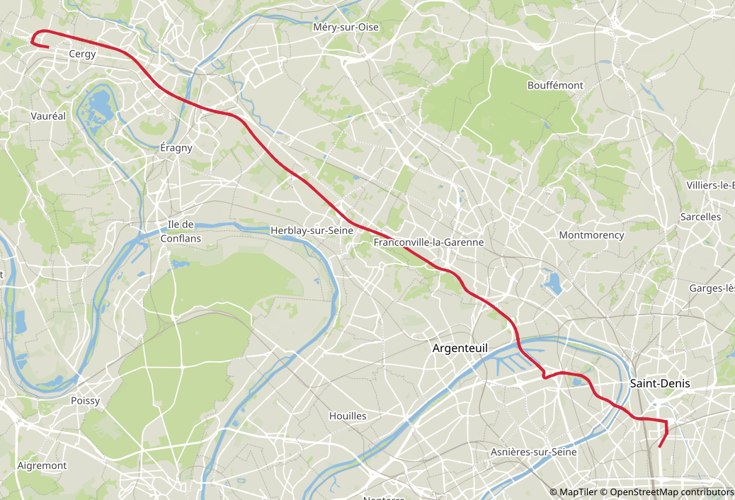
Earliest-arrival query
- Input: Origin (Cergy); Destination (Saint-Denis); Departure-time (8 a.m.)
-
Output:
Arrival time: 9:10 a.m.
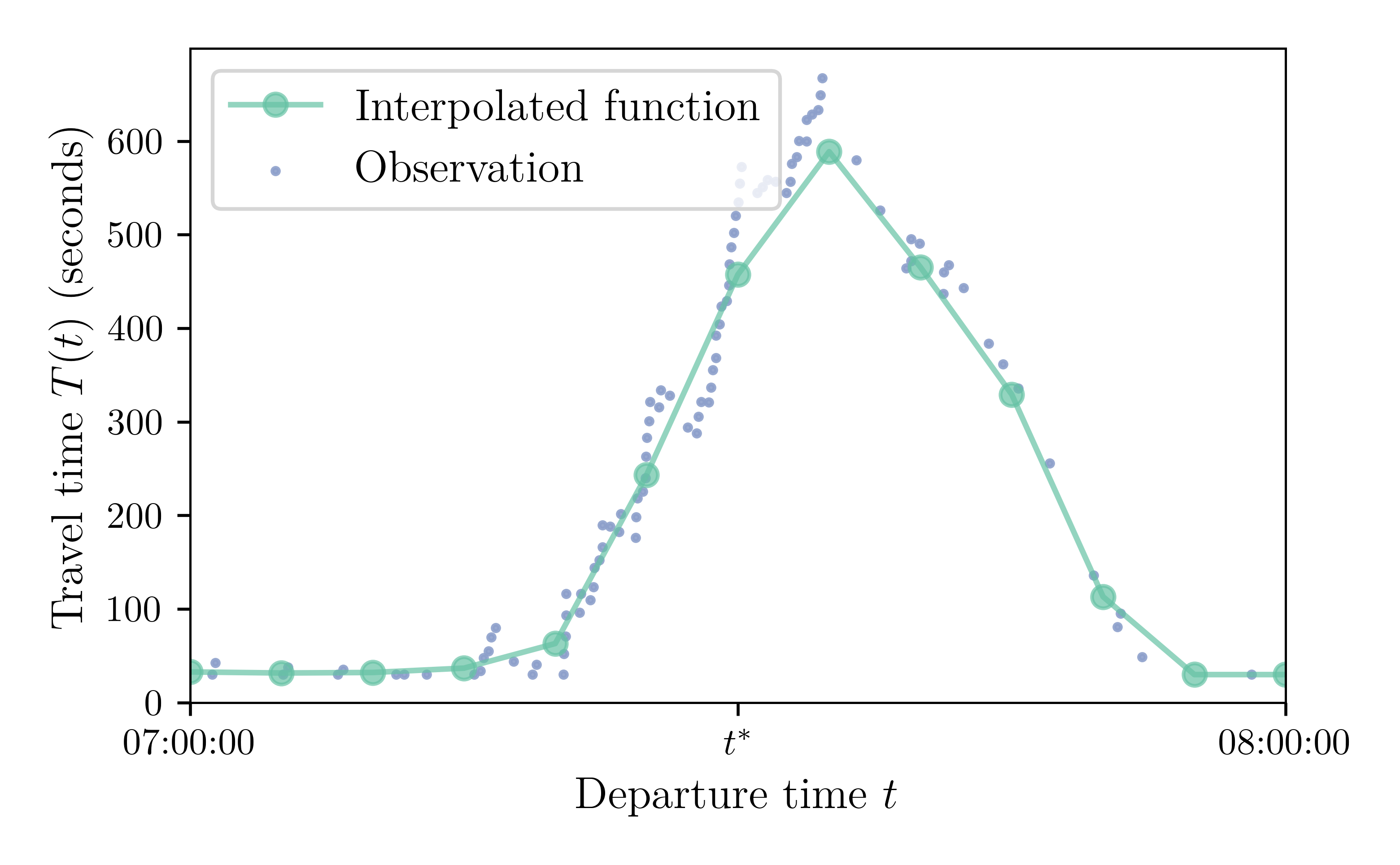
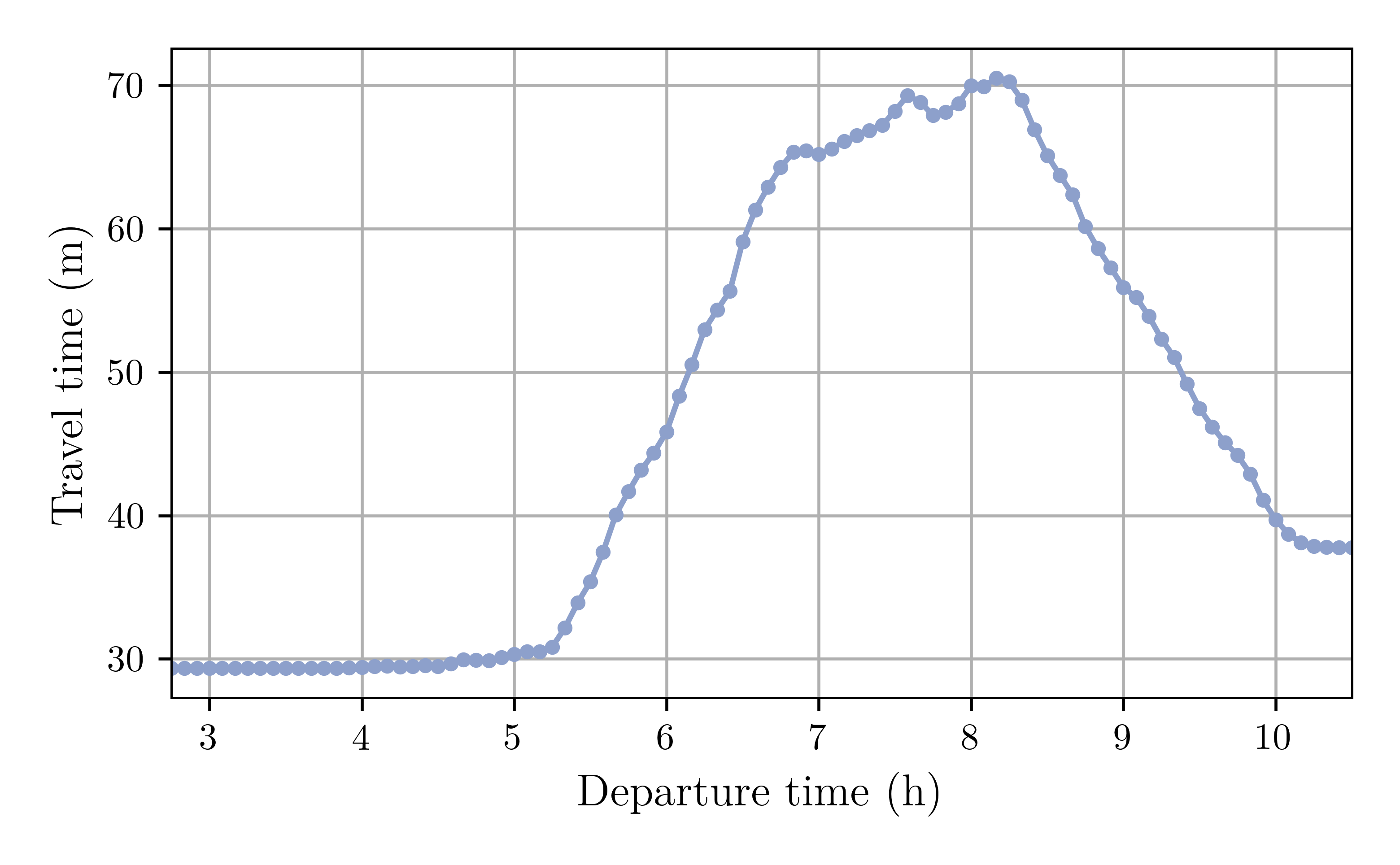
Profile query
- Input: Origin (Cergy); Destination (Saint-Denis)
-
Output:
Using Routing Algorithms
- The routing algorithms of METROPOLIS2 can be used independently from the simulator: "Run routing" button on the GUI version or "routing_cli" executable on the CLI version
-
Four input files:
- Parameters (JSON)
- Queries (CSV or Parquet)
- Edges (CSV or Parquet)
- [Optional] Edges' travel-time functions (CSV or Parquet)
-
Three output files:
- Earliest-arrival query results (CSV or Parquet)
- Profile query results (CSV or Parquet)
- Running times (JSON)
Edges Input File
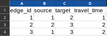
- Similar format than the Edges input file of METROPOLIS2
- Column
travel_time: constant travel time on the edge
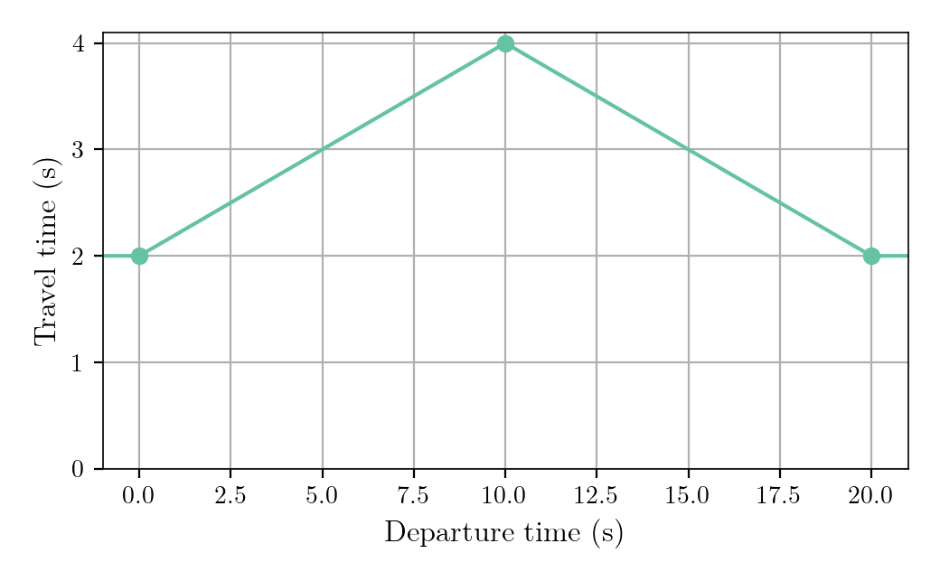
Edges' TTF Input File
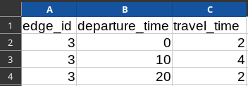
- Specify for some edges the travel-time function to be used instead of the constant travel time
- The travel-time function is given as a list of breakpoints (departure time, travel time)
- Format very similar to METROPOLIS2's output file for road-network conditions
Queries Input File
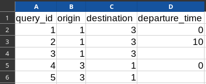
query_id: Identifier of the query (used in the results)origin: Identifier of the origin nodedestination: Identifier of the destination nodedeparture_time: Departure time from origin- If departure time is omitted: profile query; otherwise: earliest-arrival query
Routing Parameters JSON File
						{
							"input_files": {
								"queries": "queries.csv",
								"edges": "edges.csv",
								"edge_ttfs": "edge_ttfs.csv"
							},
							"output_directory": "output",
							"saving_format": "CSV"
							"algorithm": "TCH",
							"output_route": true,
							"nb_threads": 8,
						}
input_files: Path to the three input files (absolute or relative to the "parameters.json" file)output_directory: Path to the output directory (absolute or relative to the "parameters.json" file)saving_format: "CSV" or "Parquet"algorithm: "Best", "TCH", "Intersect", or "Dijkstra"output_route: Whether to compute and return the fastest paths (only for earliest-arrival queries, incompatible with "Intersect")nb_threads: Number of threads to use when running (Default is to use the maximum available)
Earliest-Arrival Queries Results
-
File
ea_results.csv(or .parquet):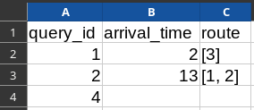
-
Input graph:
-
Input files:
Profile Queries Results
-
File
profile_results.csv(or .parquet):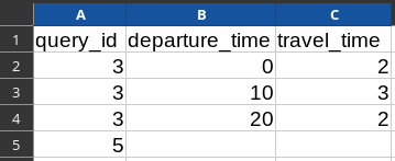
-
Input graph:
-
Input files:
Beyond Earliest Arrivals
- When all the edges' travel-time functions are constant, the time-dependent routing algorithm is equivalent to a static routing algorithm
- The
travel_timevalues can be set to something else (e.g., edge's length) and the algorithm will minimize with respect to this metric - To compute the length of the shortest path, set the values to the edges' length and run earliest-arrival queries with a departure time of 0
Session 2 Task
- Create input edges and vehicle-types files (toy network or large-scale network with OpenStreetMap import)
- Run the routing algorithm on your road-network (e.g., retrieve shortest path distances for a set of origin-destination pairs)