METROPOLIS2 Course
Session 1: Introduction
Lucas Javaudin
Spring 2024
Plan of this Session
- Course organization
- Overview of METROPOLIS2
- Getting started with METROPOLIS2
- Task for next session
Sessions
- Introduction (13th March)
- Supply side: road network (27th March)
- Demand side: agents, travel alternatives and trips
- Technical parameters and running the simulator
- Reading and understanding the results
- Case-study: Paris' low-emission zone (Input)
- Case-study: Paris' low-emission zone (Output)
- Extensions: fuel consumption, CO2 emissions and local pollutants
General Information
- The session's slides are sent to all participants at the end of the session
- One task wil be proposed at the end of each session (to be done for the next session)
- Tasks are optional but highly recommended: Practice makes perfect
- Any participant who completes all the tasks and writes a 2-page report can get an attendance certificate
A Bit of History
- 1997-2009: Simulator METROPOLIS1 [C++] (de Palma, Marchal, Nesterov)
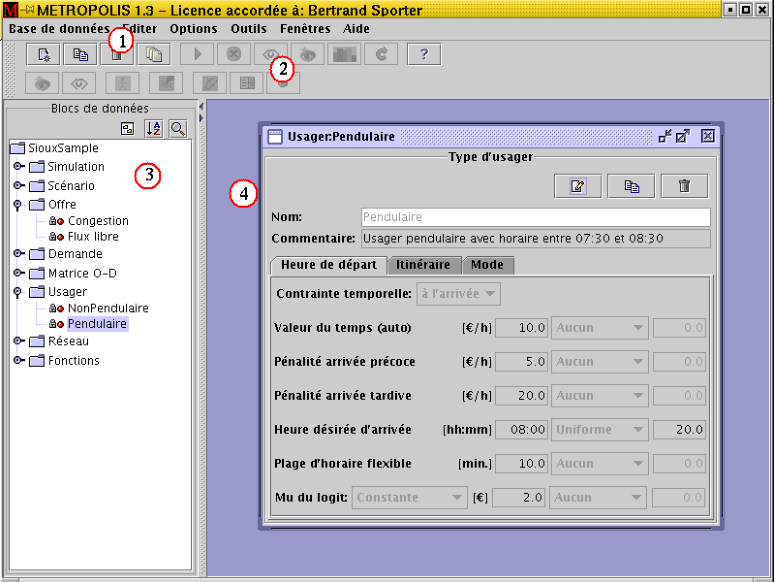
- 2001-2009: Interface for METROPOLIS1 [Java] (Marchal)
- 2018-2021: Web interface for METROPOLIS1 [Python Django] (Javaudin)
- 2021-: METROPOLIS2 [Rust] (de Palma, Javaudin)
What is METROPOLIS2
Transport simulator with the following characteristics:
- Agent-based
- Multi-modal
- Micro-founded
- Dynamic
- Adapted for small- and large-scale simulations
- Fast
- Extensible
General Flow

- Python scripts are used to convert data to the simulator's input files
- The METROPOLIS2 simulator reads the input files and writes output files (Parquet or CSV format)
- Python scripts are used to read the output files and produce results
Python scripts can be shared between users or replaced by other tools
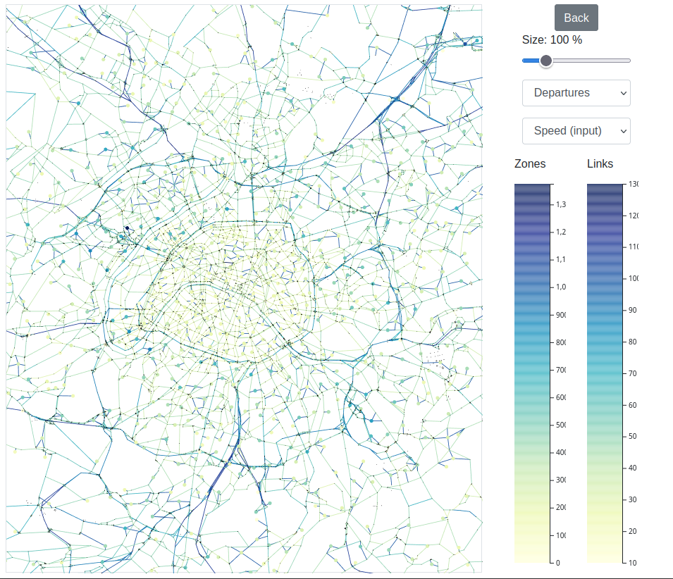
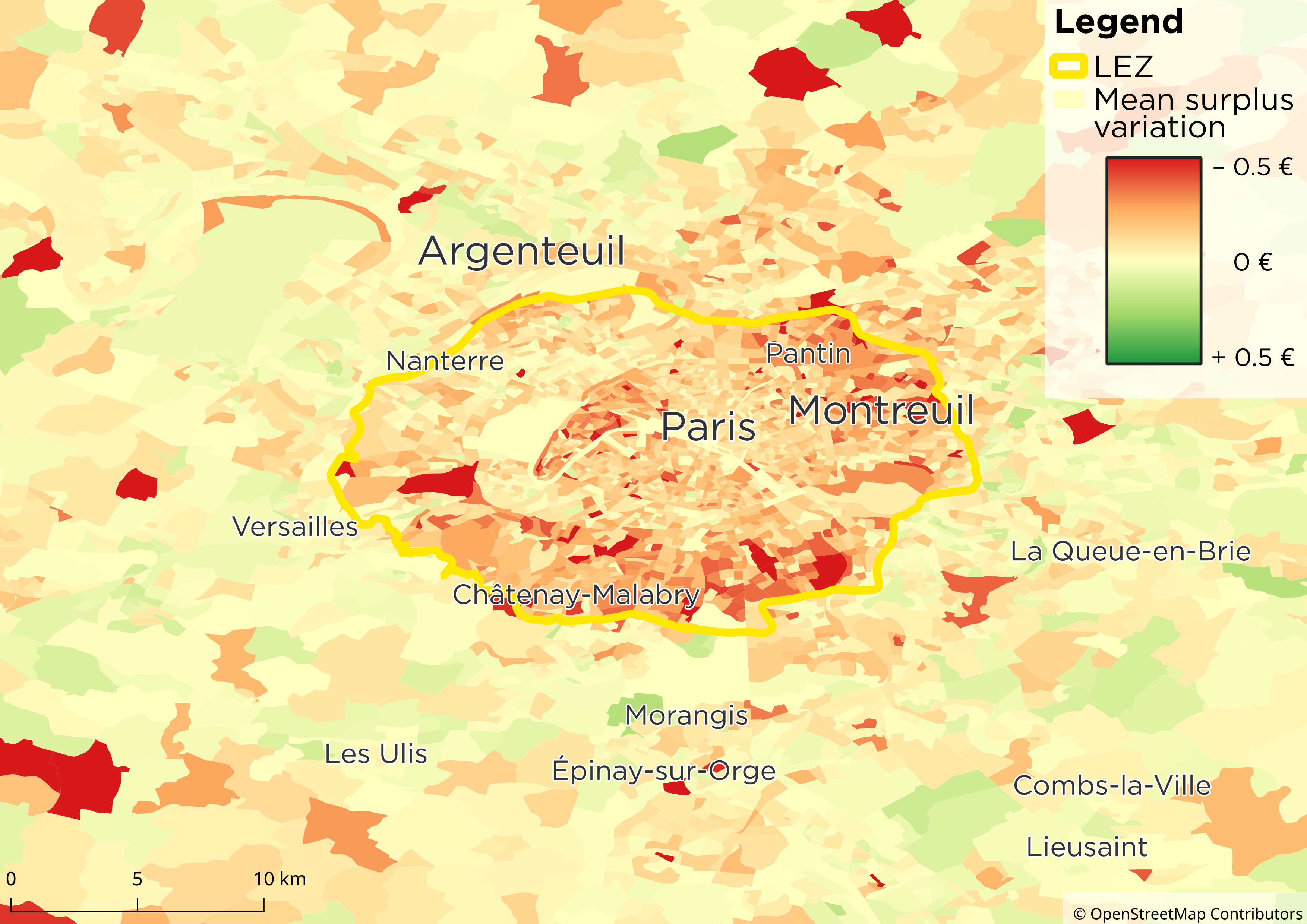
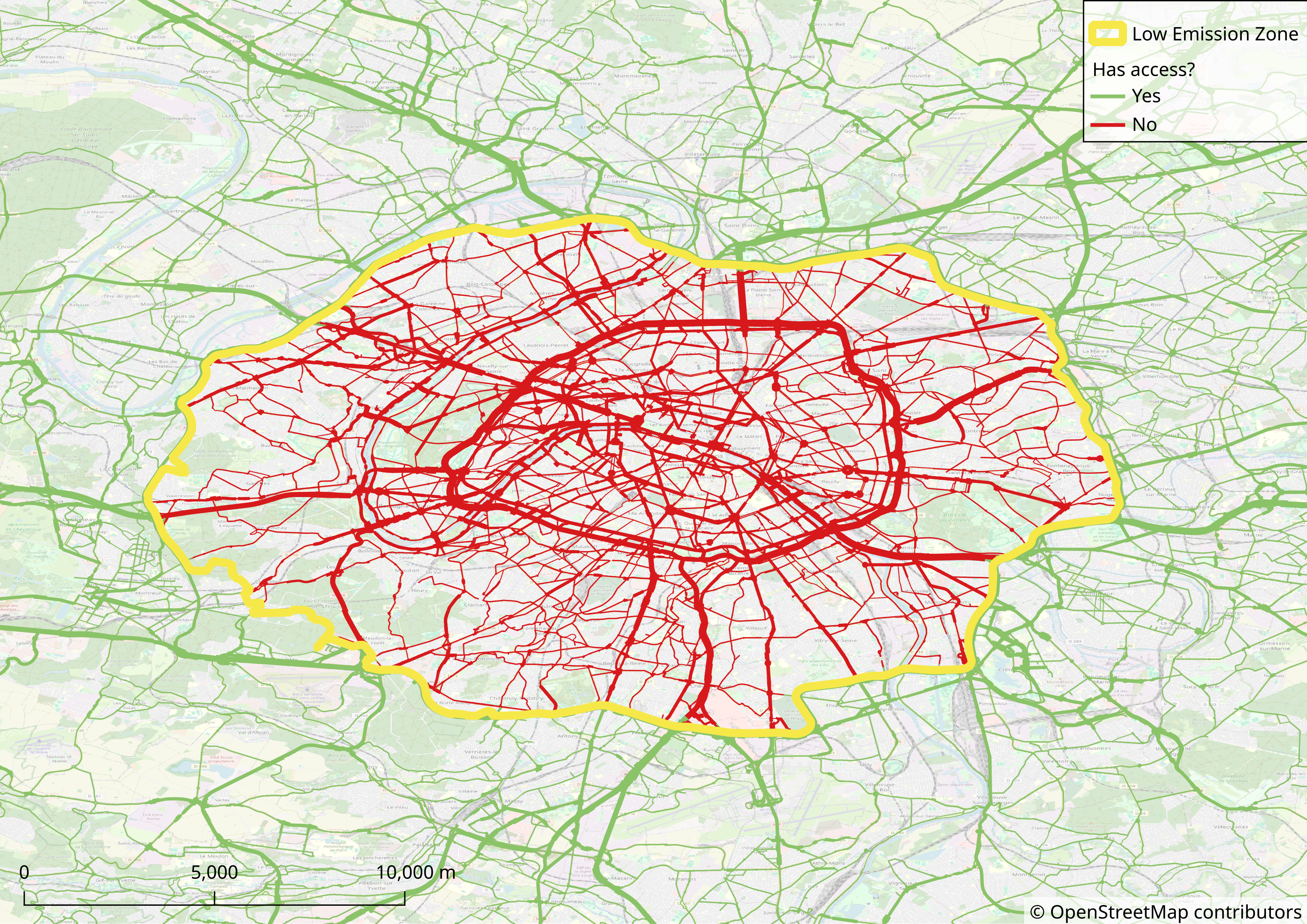
Examples of Productions
Travel surplus variation at the IRIS level when Paris's Low Emission Zone is implemented
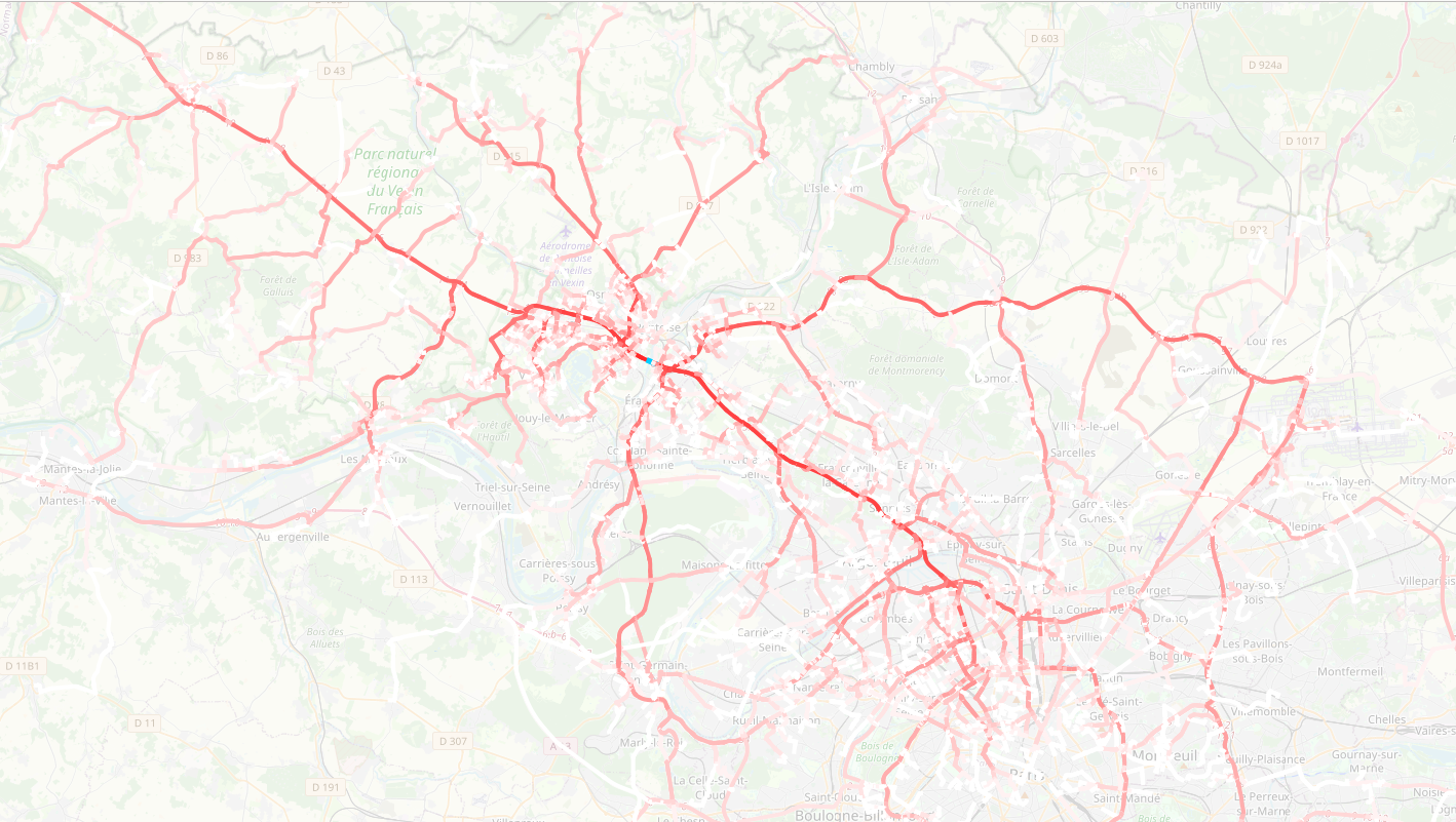
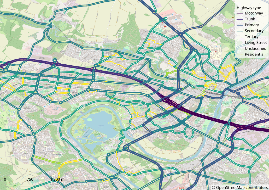
Car flows for all trips going through highway A15 near Cergy
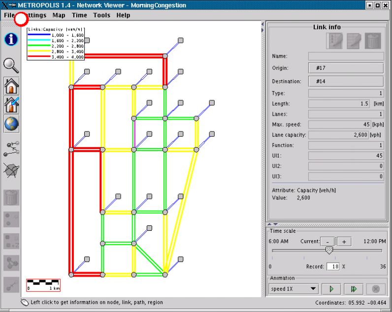
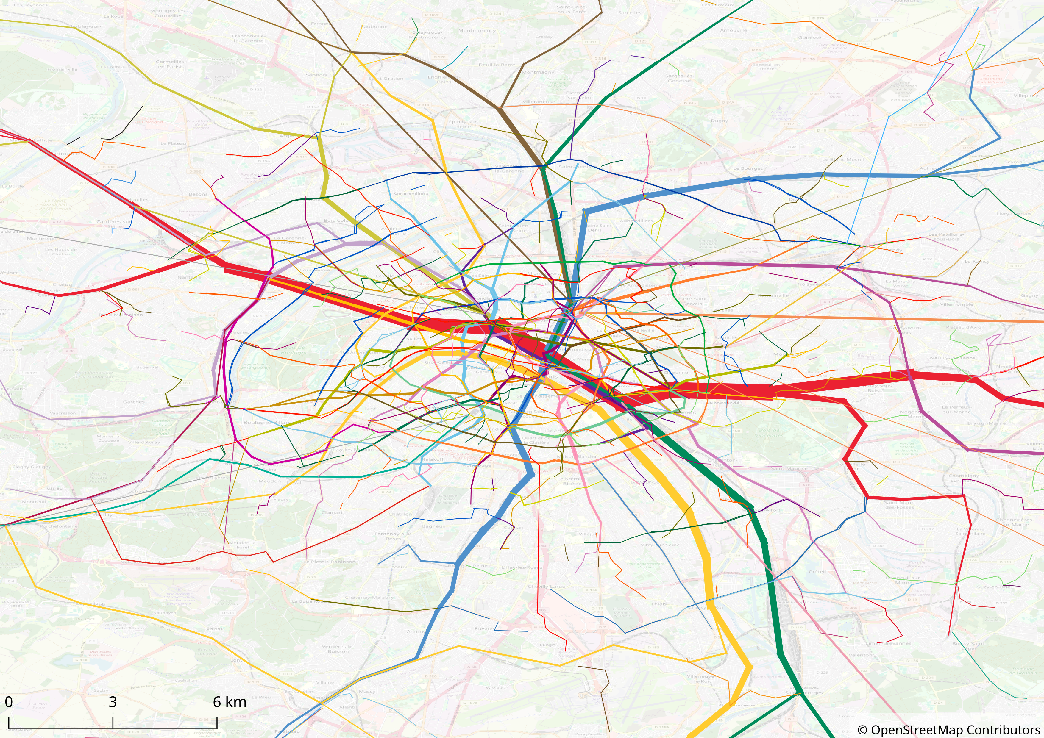
Public-transit flows by line, Paris' urban area, Morning peak
Vehicle movements in the surroundings of Cergy, 08:00 to 08:05
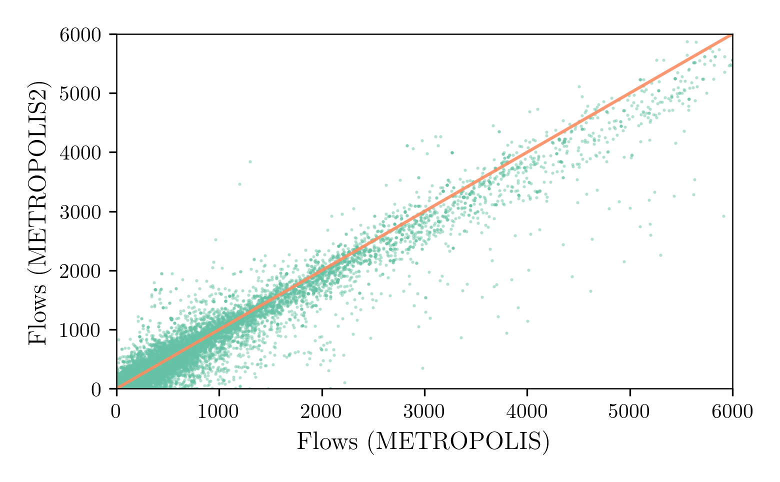
Comparison with METROPOLIS1
- Point-to-point trips (vs OD matrix)
- Trip chaining
- More flexible utility and choice models specifications
- Full heterogeneity
- Improvement congestion modeling
- Different vehicle types (including speed limit and road restrictions)
- No en-route route choice
- No proper toll implementation
- No incidents
Comparison with METROPOLIS1
Comparison with MATSim
| METROPOLIS2 | MATSim |
|---|---|
| Trip-based | Activity-based |
| Exogenous activity duration | Endogenous activity duration |
| Flexible utility specification | Charypar-Nagel utility function |
| CSV / Parquet input | XML input |
| Discrete-choice theory | Co-evolutionary algorithm |
- Discrete-choice theory: choice among all alternatives, based on discrete-choice models (e.g., Logit)
- Co-evolutionary algorithm: choice in a limited subset of alternatives
The Bottleneck Model
-
A road is connecting an origin $A$ to a destination $B$: free-flow travel time is $t^f$ and there is a point-bottleneck of capacity $s$
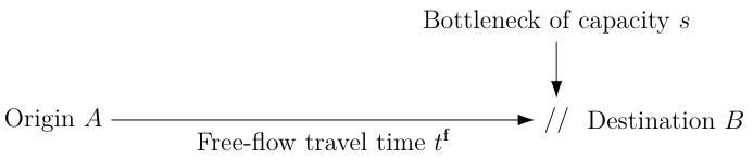
- Travel time from $A$ to $B$ is \[ t^f + \frac{Q(t + t^f)}{s} \] with $Q$ the length of the bottleneck queue at time $t$.
The Bottleneck Model
- $N$ agents are traveling from Origin $A$ to Destination $B$
- Utility is given by \[ V(t) = -\alpha \cdot T(t) - \beta \cdot [t^* - t - T(t)]_+ - \gamma \cdot [t + T(t) - t^*]_+ \]
- Agents choose the departure time maximizing utility (Arnott, de Palma and Lindsey, 1990): \[ t^d = \arg \max V(t) \]
- Agents choose departure time $t$ with probability (Continuous Logit, de Palma, Ben-Akiva, Lefevre and Litinas, 1983): \[ p(t) = \frac{e^{V(t) / \mu}}{\int_{t^0}^{t^1} e^{V(\tau)/\mu} d \tau} \]
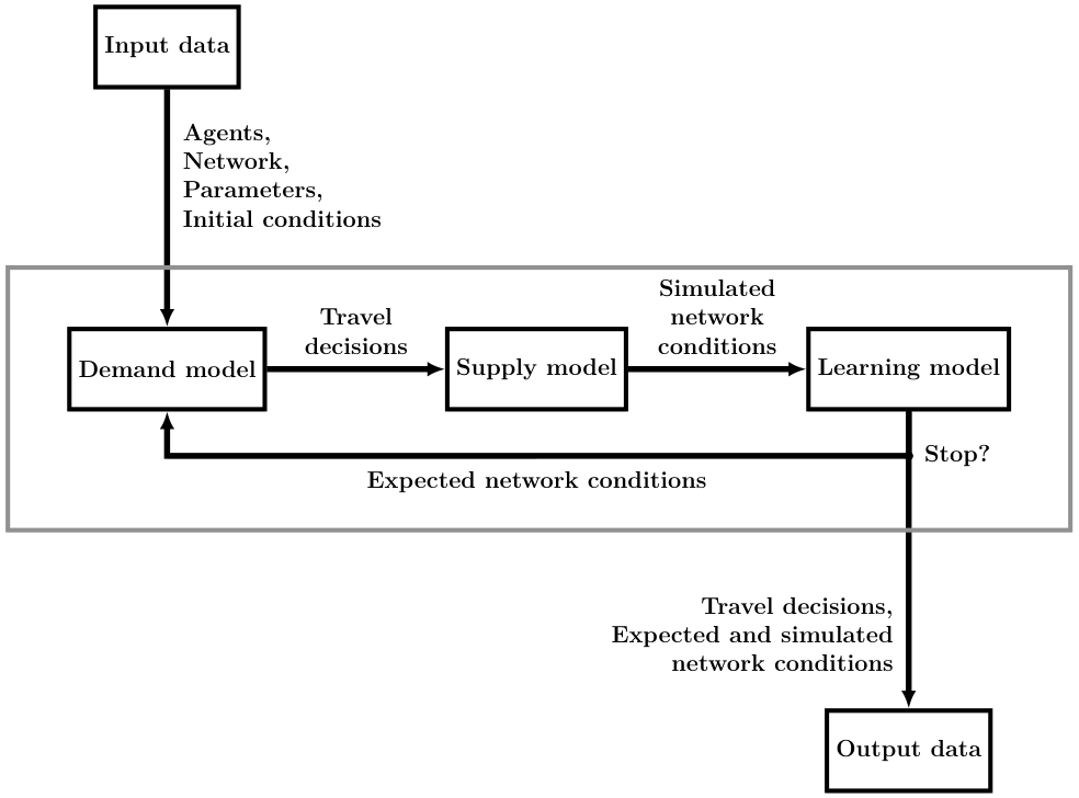
METROPOLIS2 Fundamental Flow Diagram
Input Data
- Population: $N = 100,000$ agents, $\alpha$-$\beta$-$\gamma$ preferences ($\alpha = 10\$ / h$, $\beta = \gamma = 5\$ / h$, $t^*$ = 7:30 a.m.)
- Road network: Single road, free-flow travel time $t^f$ = 30 seconds, bottleneck of capacity $s = 150,000$ cars / h
- Initial network conditions: free flow
METROPOLIS2 Fundamental Flow Diagram
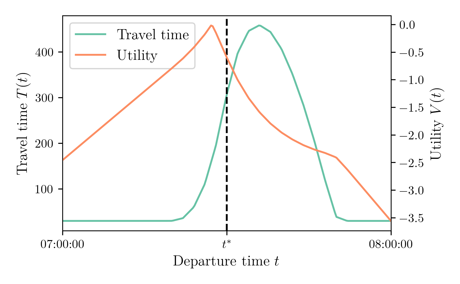
Demand Model: Computing Utility
We start from constant free-flow travel-time function and compute the utility function \[ V(t) = -\alpha \cdot T(t) - \beta \cdot [t^* - t - T(t)]_+ - \gamma \cdot [t + T(t) - t^*]_+ \]
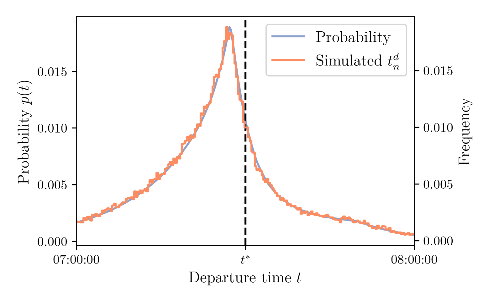
Demand Model: Computing Departure-Time Probability
The departure-time probabilities are computed from the Continuous Logit formula \[ p(t) = \frac{e^{V(t) / \mu}}{\int_{t^0}^{t^1} e^{V(\tau)/\mu} d \tau} \]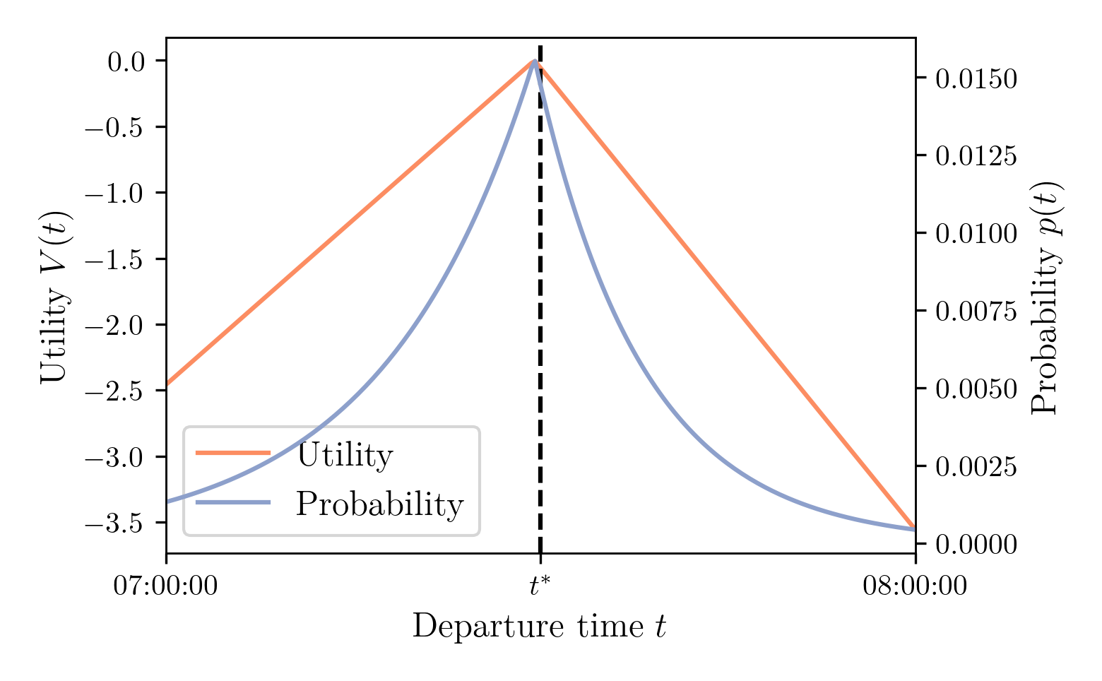
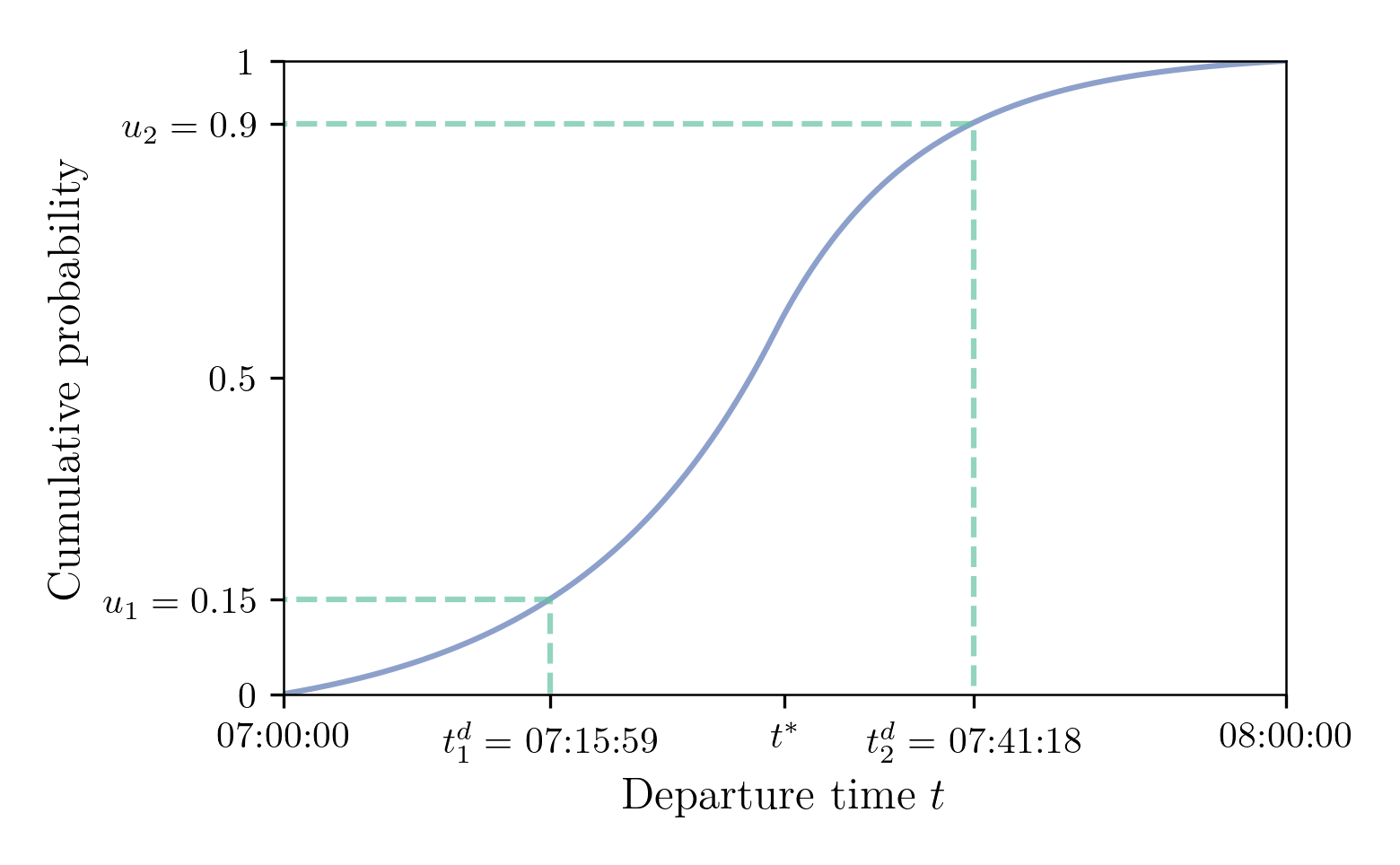
Demand Model: Simulating Departure Times
How to draw departure times from the probability function?
Inverse transform sampling: $t^d = F^{-1}(u)$ with $u \sim \mathcal{U}([0, 1])$ and $F^{-1}$ the CDF
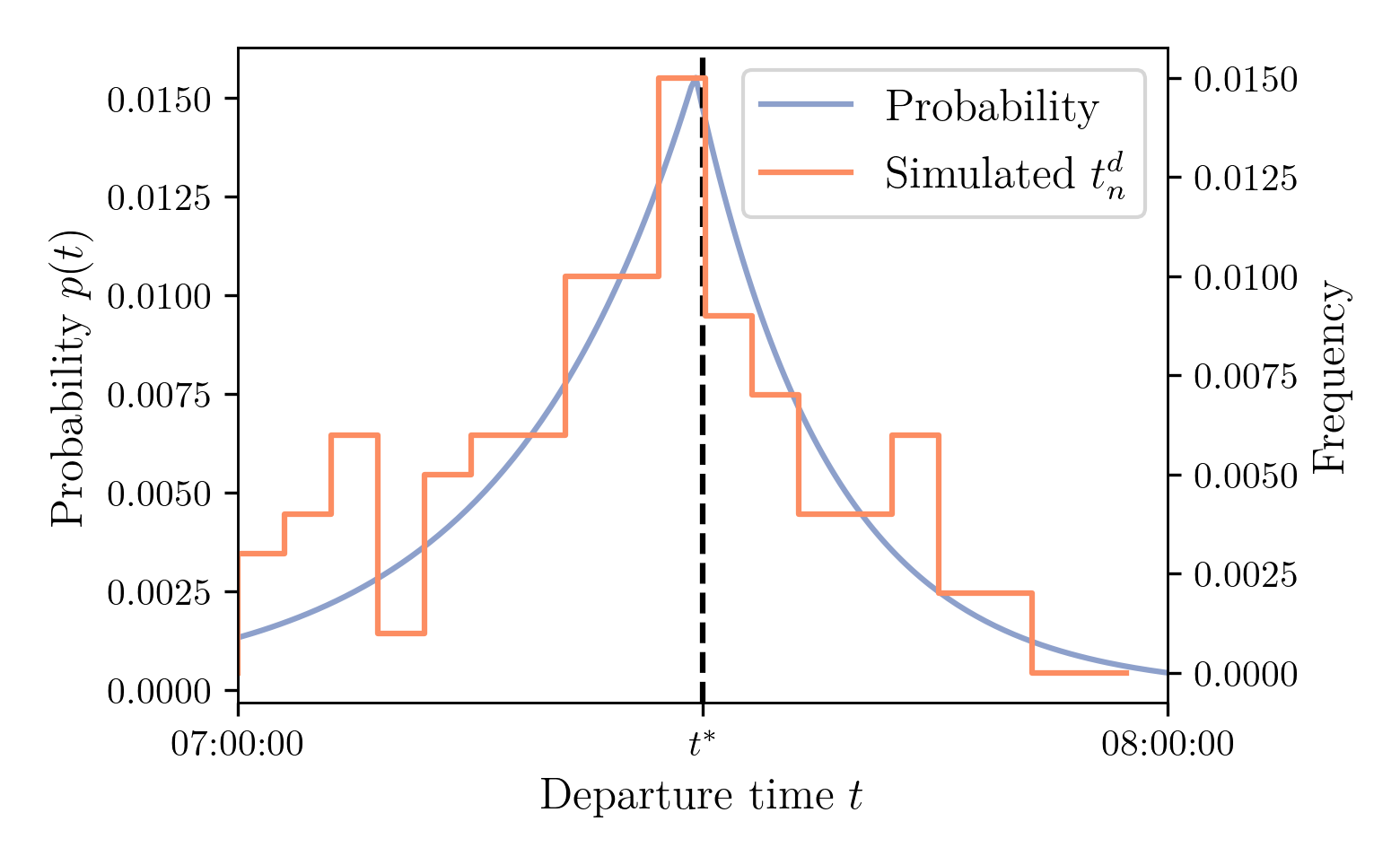
Demand Model: Simulated Departure Time Distribution
Draws with $N = 100$
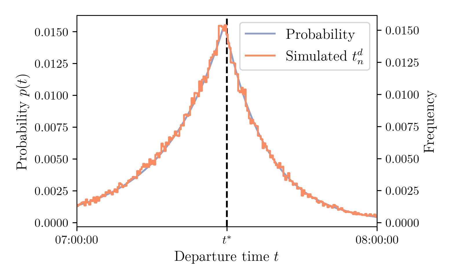
Demand Model: Simulated Departure Time Distribution
Draws with $N = 100,000$
METROPOLIS2 Fundamental Flow Diagram
Supply Model: Simulating Bottlenecks
- Bottleneck capacity: \[ \text{900 cars / hour} \Leftrightarrow \text{0.25 car / second} \Leftrightarrow \text{4 seconds / car} \]
- Departure times: $[1, 6, 7, 9]$
- T1: Agent 1 enters the bottleneck, leaves immediately, bottleneck closed until T5
- T5: Bottleneck opens
- T6: Agent 2 enters the bottleneck, leaves immediately, bottleneck closed until T10
- T7: Agent 3 enters the bottleneck, pushed to the queue
- T9: Agent 4 enters the bottleneck, pushed to the queue
- T10: Bottleneck opens, agents 3 leaves, bottleneck closed until T14
- T14: Bottleneck opens, agents 4 leaves, bottleneck closed until T18
- T18: Bottleneck opens
Supply Model: Bottleneck Properties
- Bounded by the capacity: The outflow of the bottleneck cannot exceed its capacity
- FIFO: The cars exit the bottleneck in the same order that they entered it
- Continuous time: It can work with very small or very large capacities
Supply Model: Simulated Departure and Arrival Time Distributions
$N = 100,000$, Capacity 150,000 cars / hour or 41.67 cars / second or 0.024 second / car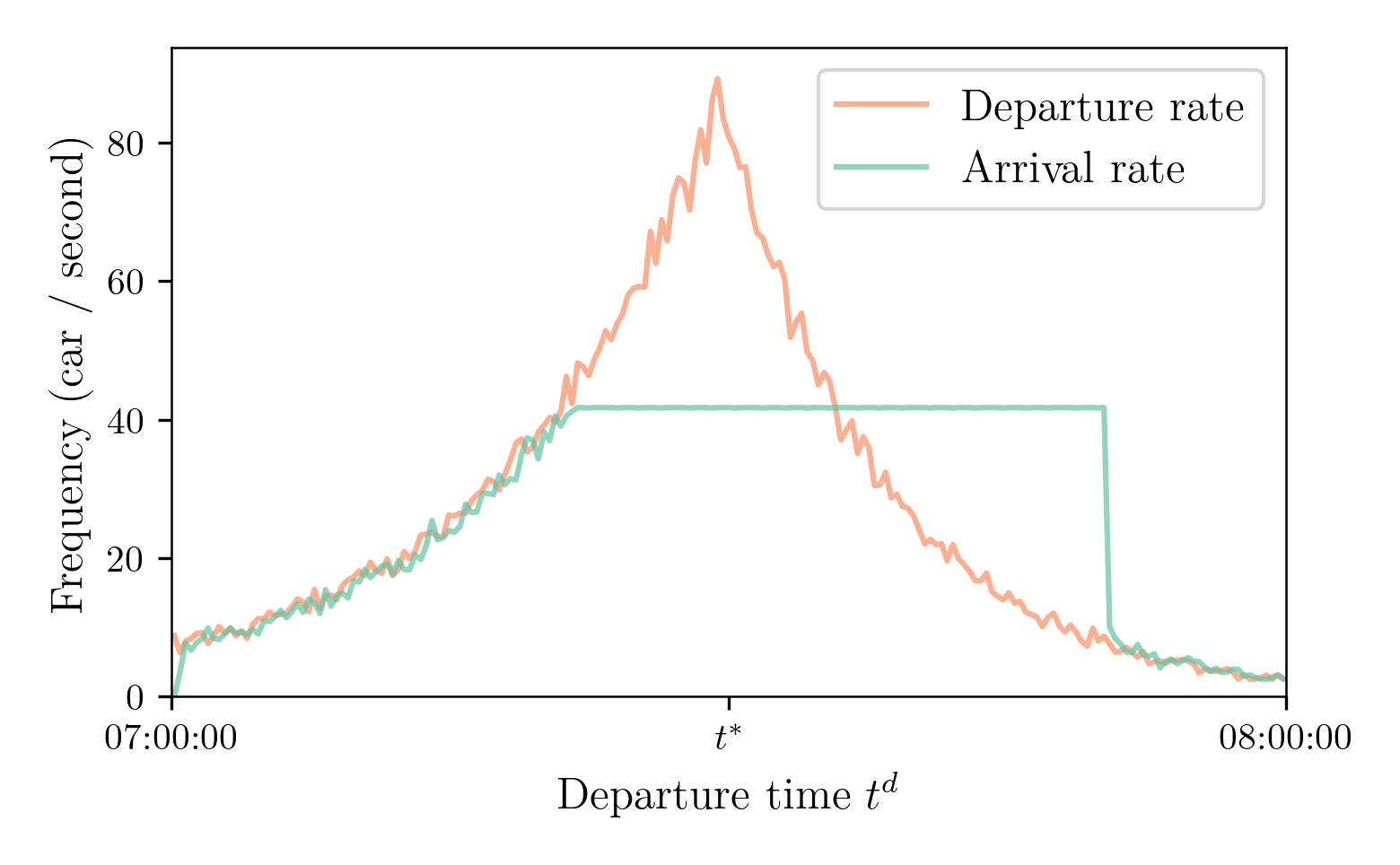
Supply Model: Simulated Travel Times
$N = 100,000$, Capacity 150,000 cars / hour or 41.67 cars / second or 0.024 second / car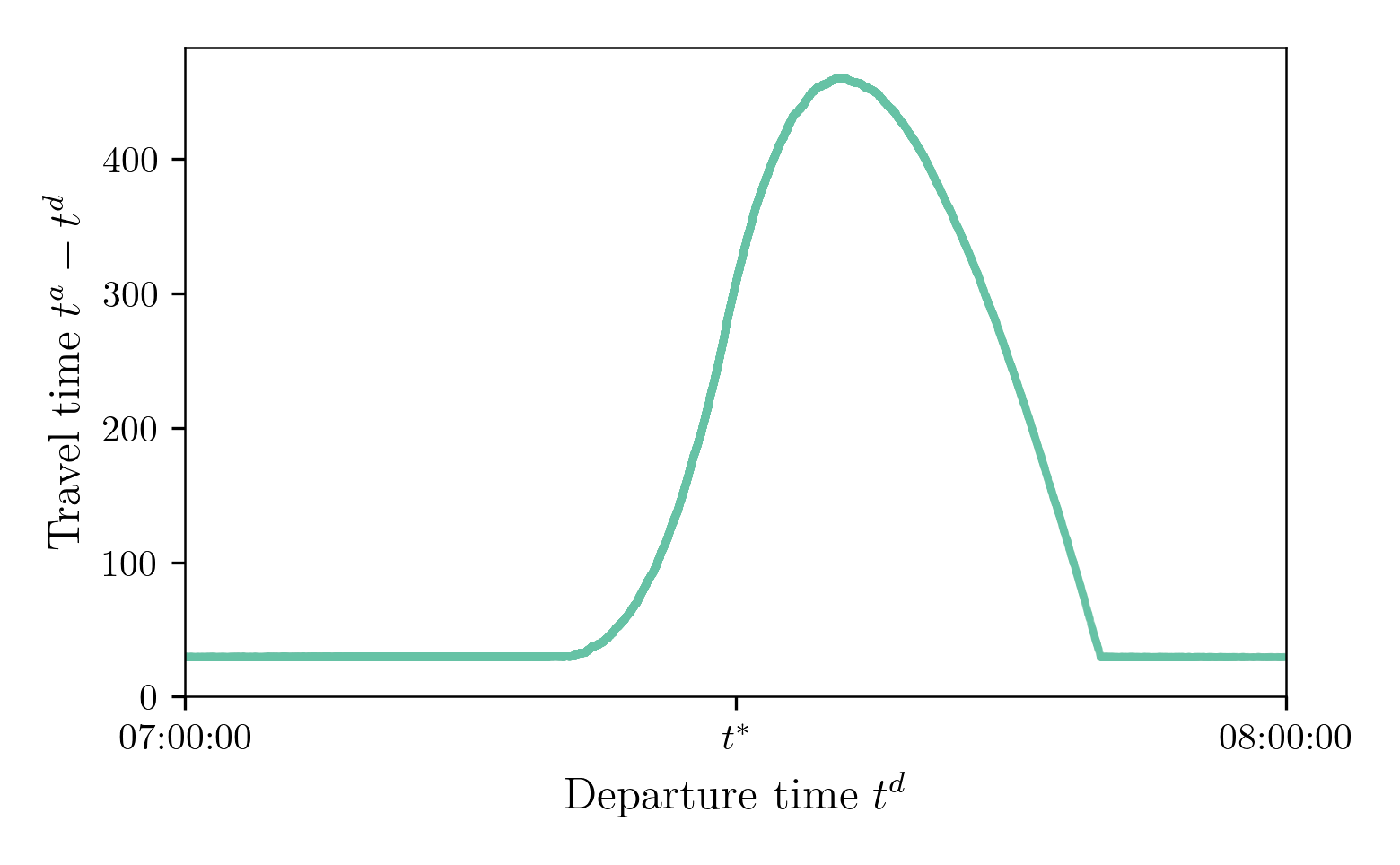
Supply Model: Simulated Travel Times
$N = 100$, Capacity 150 cars / hour or 0.04167 cars / second or 24 seconds / car
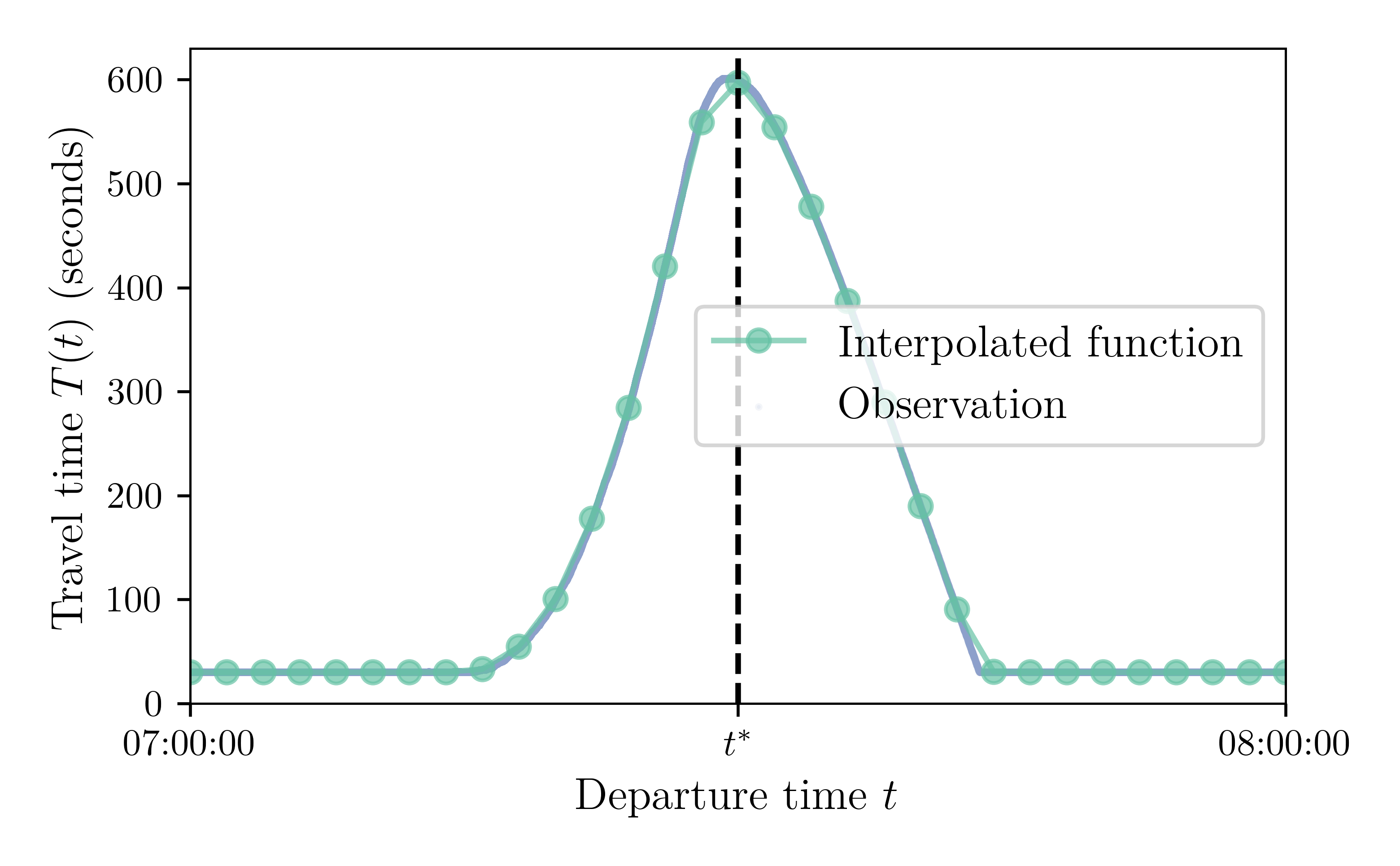
Supply Model: Piecewise-Linear Travel-Time Function
How to build the travel-time function from the simulated points? Linear interpolation!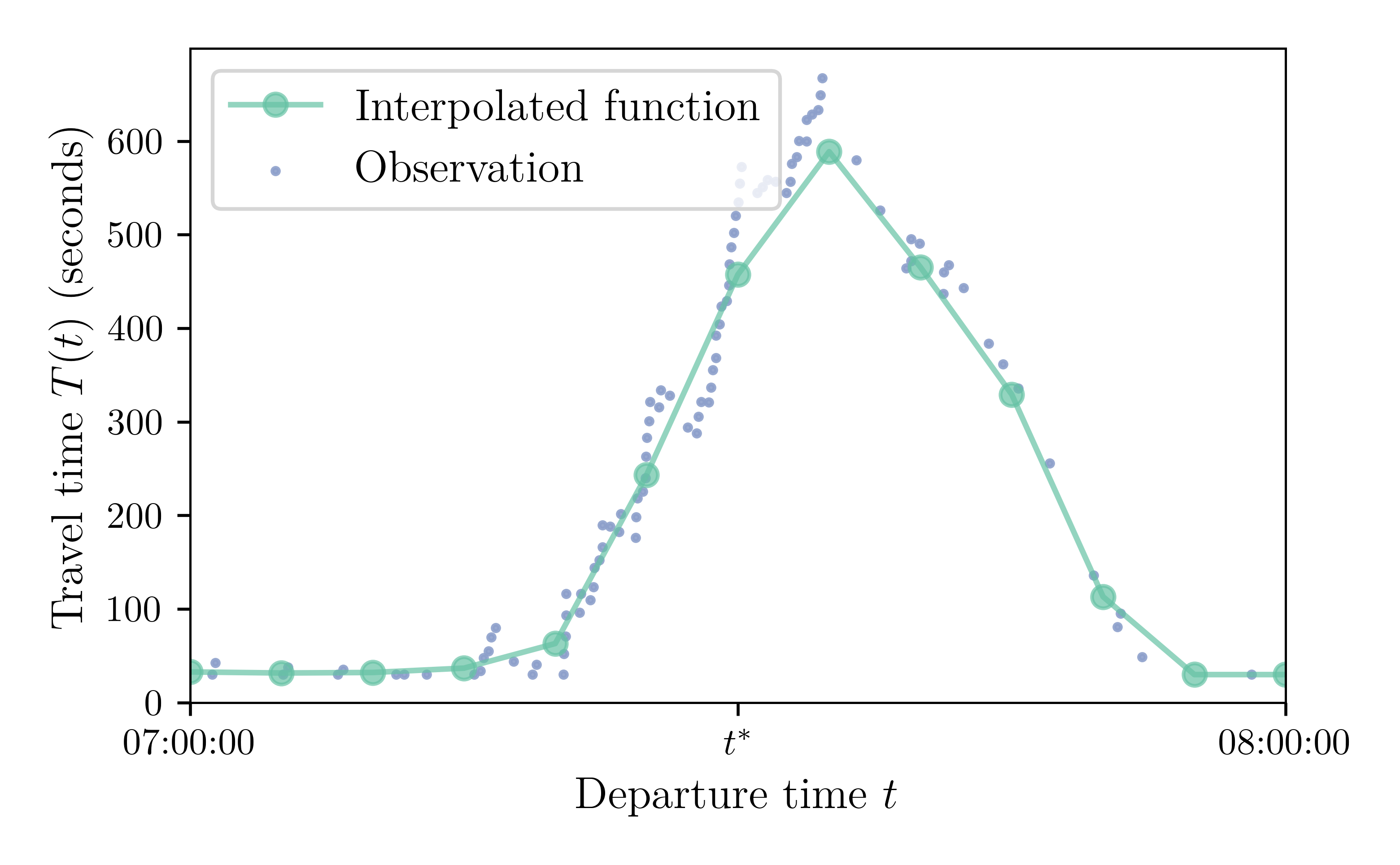
$N = 100$, Capacity 150 cars / hour or 0.04167 cars / second or 24 seconds / car
Supply Model: Piecewise-Linear Travel-Time Function
5-minute breakpoints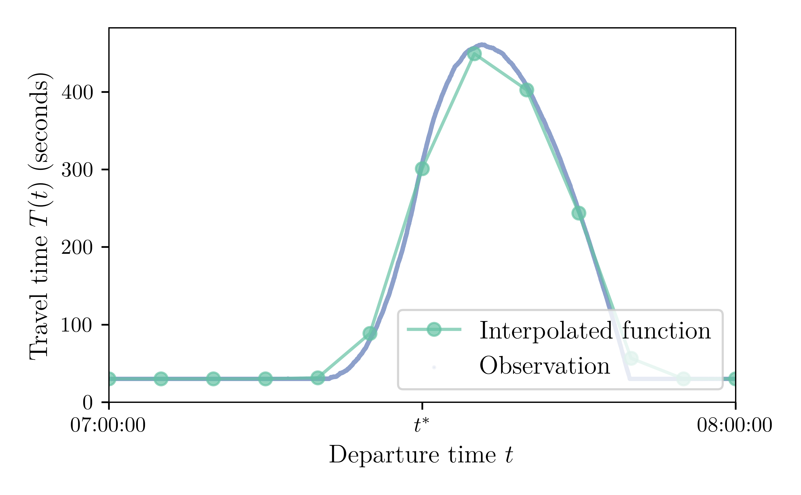
$N = 100,000$, Capacity 150,000 cars / hour or 41.67 cars / second or 0.024 second / car
Supply Model: Piecewise-Linear Travel-Time Function
2-minute breakpoints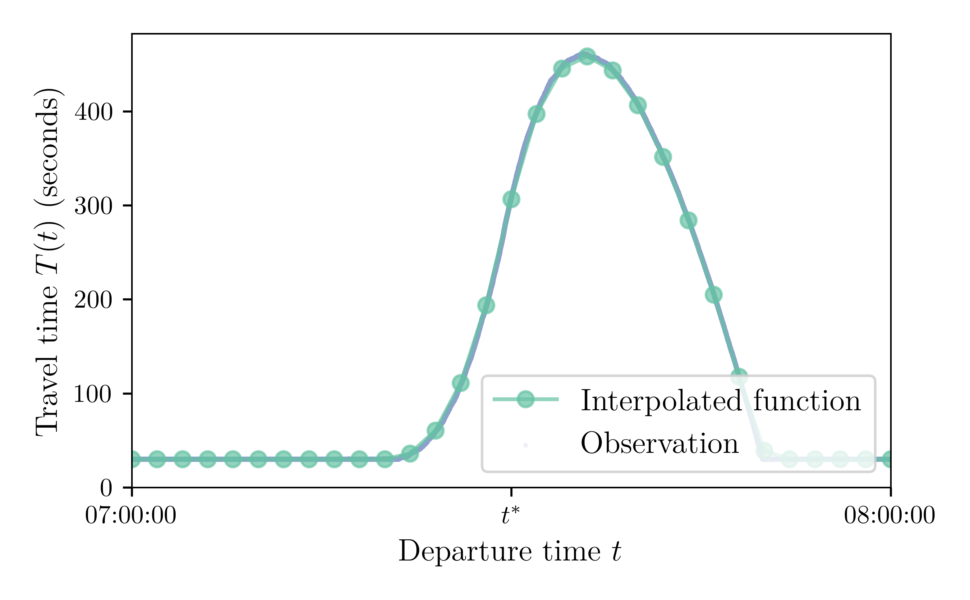
$N = 100,000$, Capacity 150,000 cars / hour or 41.67 cars / second or 0.024 second / car
Summary
Inconsistency / Non-equilibrium: The travel-time function used to simulate the departure times (in the demand model) does not match the travel-time function resulting from these departure times (in the supply model)
Nash equilibrium definition: No agent can increasing their utility by choosing another departure time, given the other agents' departure times
"Naive" METROPOLIS2
(TTF = travel-time function)
-
$\hat{T}$: Expected TTF, used to compute utilities in the demand model
-
$T$: Simulated TTF computed in the supply model from the chosen departure times
Naive algorithm:
- Initialization: $\hat{T} =$ free-flow TTF
- Demand model: Draw the departure times given $\hat{T}$
- Supply model: Compute $T$ resulting from the departure times
-
If $T = \hat{T}$, stop.
Otherwise, $\hat{T} \leftarrow T$ and go back to Step 2.
Second Iteration
100 Iterations
METROPOLIS2 Fundamental Flow Diagram
Learning Model
- The TTF expected for the next iteration depends on the TTF just simulated, $T$, but also on the previously expected TTF $\hat{T}$.
- At iteration $\kappa$: \[ \hat{T}_{\kappa + 1} = f(\kappa, T_{\kappa}, \hat{T}_{\kappa}) \]
- Exponential smoothing method: \[ f(\kappa, T_\kappa, \hat{T}_{\kappa}) = \lambda T_\kappa + (1 - \lambda) \hat{T}_{\kappa} \] with $\lambda \in [0, 1]$, the smoothing factor.
- With $\lambda = 1$: "naive" learning; with $\lambda = 0$: arithmetic mean.
Let's Try Again
$\lambda = 0.5$
Supply: Large Road Network
- Road network can be an arbitrary graph of nodes (intersections) and edges (road links)
- 1 bottleneck and 1 travel-time function for each edge
- Routing algorithm (Contraction Hierarchies) used to compute the travel-time function at the origin-destination level
- Route choice: the fastest route is selected
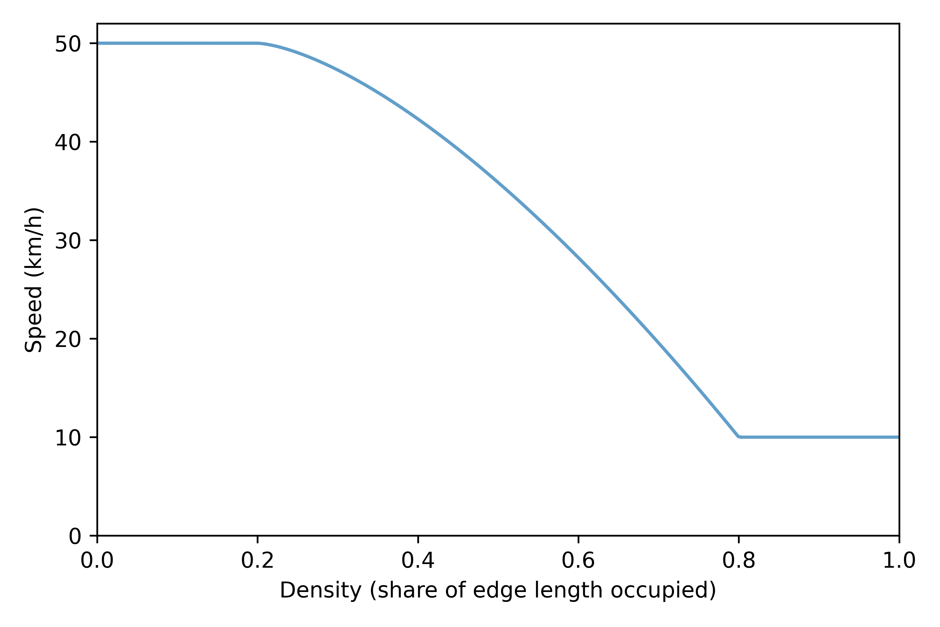
Supply: Congestion Modeling
- Speed-density function: the speed at which a vehicle travel on the road depends on the density of vehicle currently on the road
- Bottlenecks: both the inflow and outflow of a link can be limited by the bottleneck's capacity
- Queue propagation (spillback): Vehicles cannot enter a link if there is no room left; queues propagate backward at a given speed
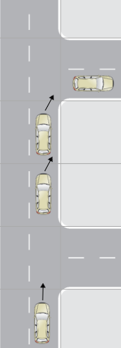
Supply: Different Vehicle Types
- Different vehicle headways and passenger car equivalents
- Different speeds / speed limits
- Different road access / road restrictions
Demand
- At the top level, agents choose among an arbitrary number of travel alternatives
- An alternative is defined as a sequence of trips and a utility function specification
- Two types of trips: road and virtual
-
The utility of an alternative is a function of:
- the travel time of each trip
- the total travel time for all the trips
- the departure time from the origin of the first trip
- the arrival time at destination of each trip
-
Choice models:
- Alternative choice: Multinomial Logit or Deterministic
- Departure-time choice: Continuous Logit or Multinomial Logit
- Almost any discrete-choice model is feasible by drawing the epsilon values (idiosyncratic chocs) "offline" and specifying them in the utility
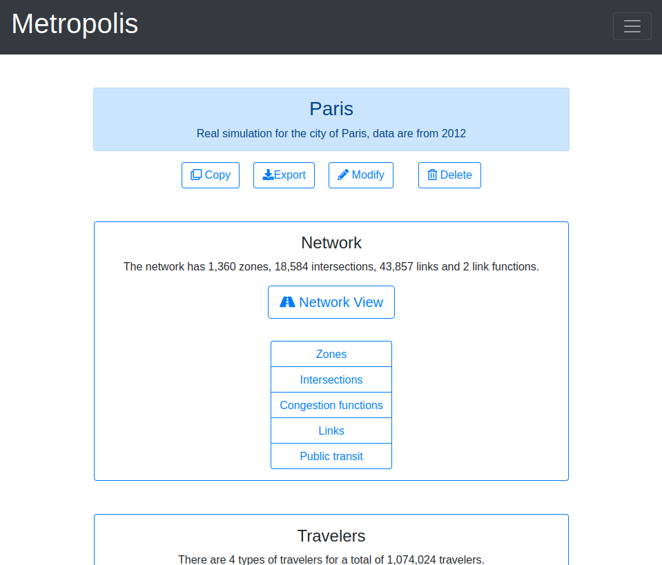
The METROPOLIS2 Website
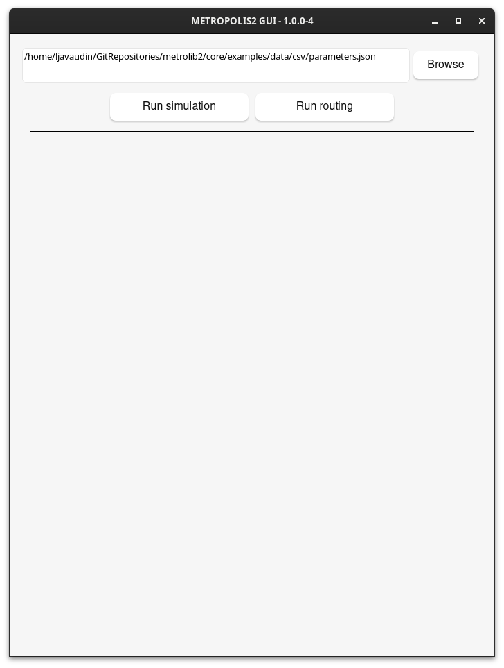
https://metropolis.lucasjavaudin.comRunning METROPOLIS2 (the Easy Way, on Windows)
- Download the last GUI version of METROPOLIS2 for Windows (tab Download on the website).
- Execute the .msi file and follow the procedure to install METROPOLIS2 (accept the non-existent risks if the antivirus complains).
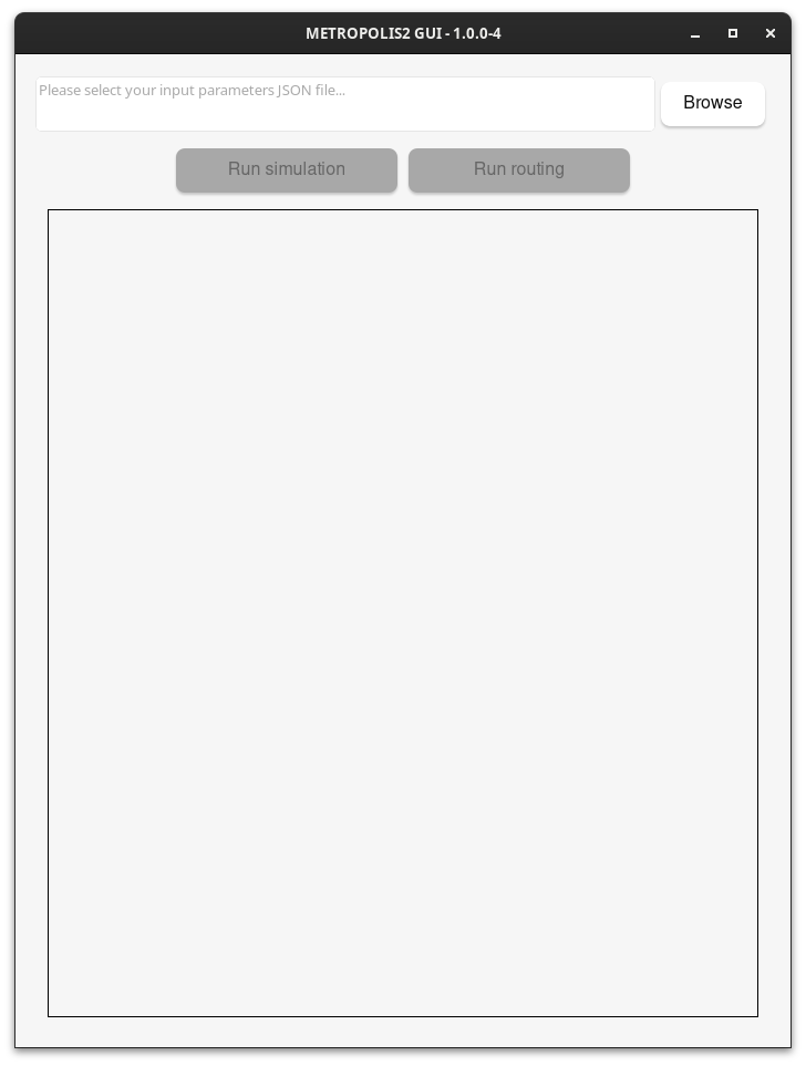
- Run the METROPOLIS2 program that is now installed on your computer.
- Click on
Browseand select yourparameters.jsonfile. - Click on the
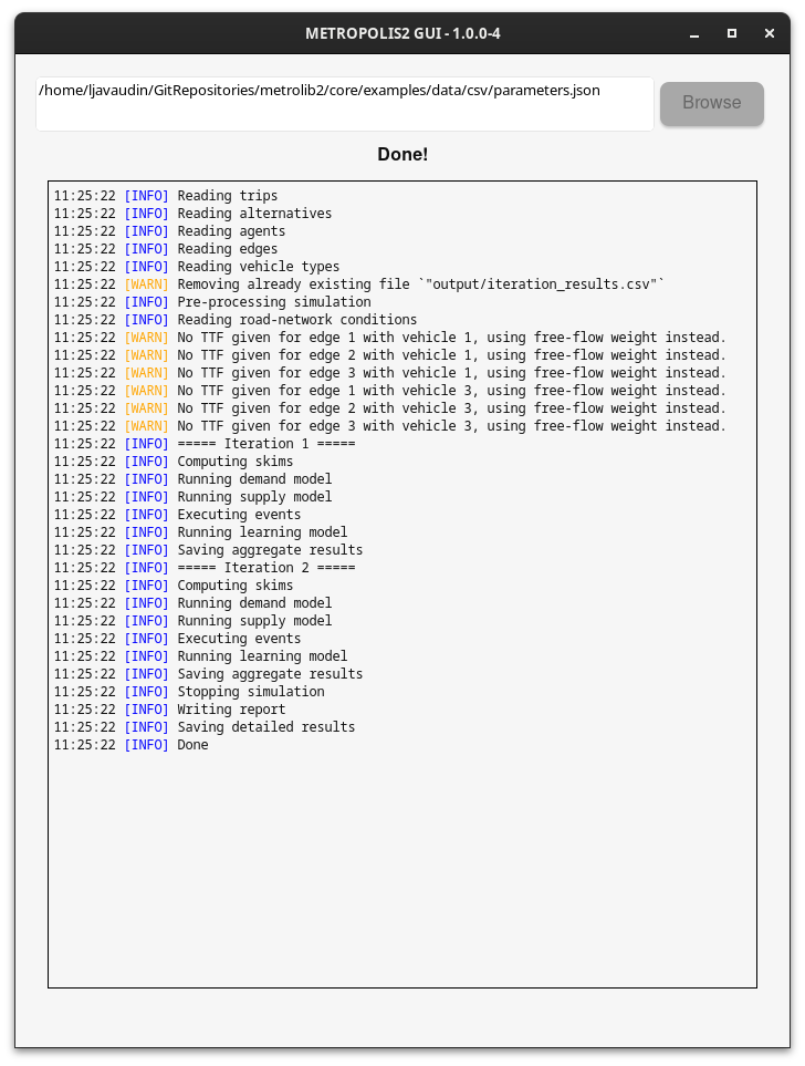
Run simulationbutton. - Check the logs and close the window when you are done.
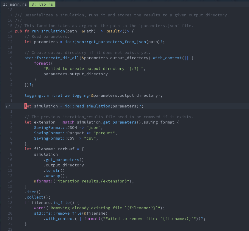
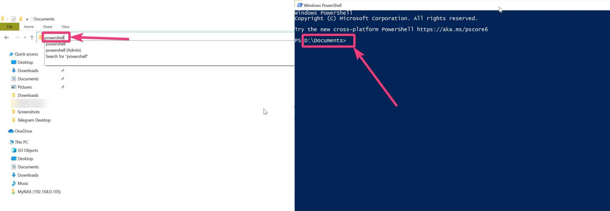
Running METROPOLIS2 (the Hard Way)
- Open a Command prompt / Terminal / Powershell with the working directory set to the location of the unzipped directory
-
For Windows, run:
.\execs\metropolis_cli.exe .\examples\data\csv\parameters.json -
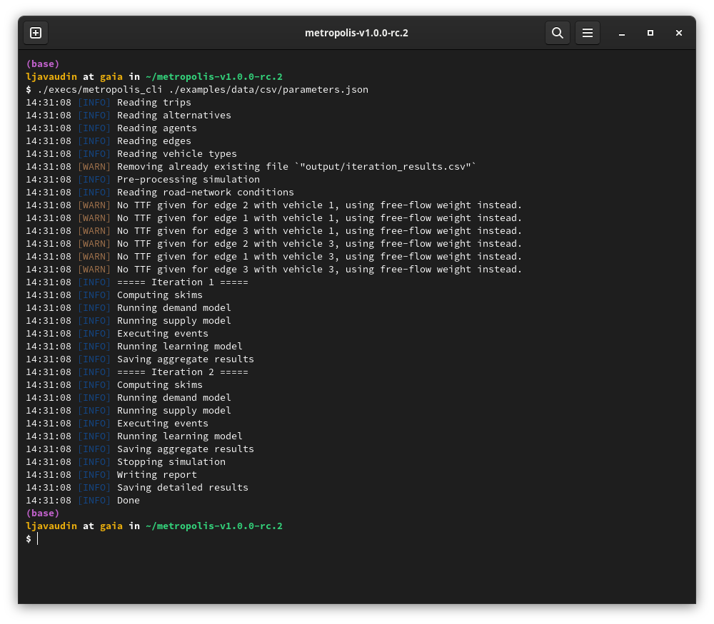
For MacOS or Linux, run:
./execs/metropolis_cli ./examples/data/csv/parameters.json - Check that the run succeeded
- The results are stored in
examples/data/csv/output/
Files Format: JSON
-
Collection of key-value pairs that can be nested indefinitely
{ "key": "value", "integer": 1, "float": 3.6, "boolean": true, "array": [ 0, 1, 2 ], "nested_array": [ {"some": "value"}, {"another": "value"} ] } - Very close to Python's
dicttype - Format used to configure the parameters of a METROPOLIS2 simulation and for some output files
- Syntax definition: https://en.wikipedia.org/wiki/JSON#Syntax
Files Format: CSV
- Row-oriented file format for tabular data
- Human readable
- Compatible with many tools and languages (including Excel!)
- Used in METROPOLIS2 for most input and output files (comma separator only)
- Recommended only for small-scale simulations, especially when using Excel
						col1,col2,col3,col4
						1,Alice,3.2,true
						2,Bob,1.4,false
						3,Charlie,2.5,false
Files Format: Parquet
- Column-oriented file format for tabular data
- Binary file (= non human-readable)
- Built-in compression: smaller file size than CSV
- Very fast
- Compatible with Python (polars or pandas libraries) and R (arrow package)
- Used in METROPOLIS2 for most input and output files
- Recommended format for large-scale simulations and people working with R or Python
						import polars as pl

						df = pl.DataFrame(
								{
										"agent_id": [0, 1, 2],
										"alt_choice.type": ["Deterministic", "Logit", "Logit"],
										"alt_choice.u": [0.3, 0.6, 0.5],
										"alt_choice.mu": [None, 0.9, 1.0],
										"alt_choice.constants": [[0.9, 1.3, 2.1], None, None],
								}
						)
						df.write_parquet("input/agents.parquet")
						In [3]: df
						Out[3]:
						shape: (3, 5)
						┌──────────┬─────────────────┬──────────────┬───────────────┬──────────────────────┐
						│ agent_id ┆ alt_choice.type ┆ alt_choice.u ┆ alt_choice.mu ┆ alt_choice.constants │
						│ ---      ┆ ---             ┆ ---          ┆ ---           ┆ ---                  │
						│ i64      ┆ str             ┆ f64          ┆ f64           ┆ list[f64]            │
						╞══════════╪═════════════════╪══════════════╪═══════════════╪══════════════════════╡
						│ 0        ┆ Deterministic   ┆ 0.3          ┆ null          ┆ [0.9, 1.3, 2.1]      │
						│ 1        ┆ Logit           ┆ 0.6          ┆ 0.9           ┆ null                 │
						│ 2        ┆ Logit           ┆ 0.5          ┆ 1.0           ┆ null                 │
						└──────────┴─────────────────┴──────────────┴───────────────┴──────────────────────┘
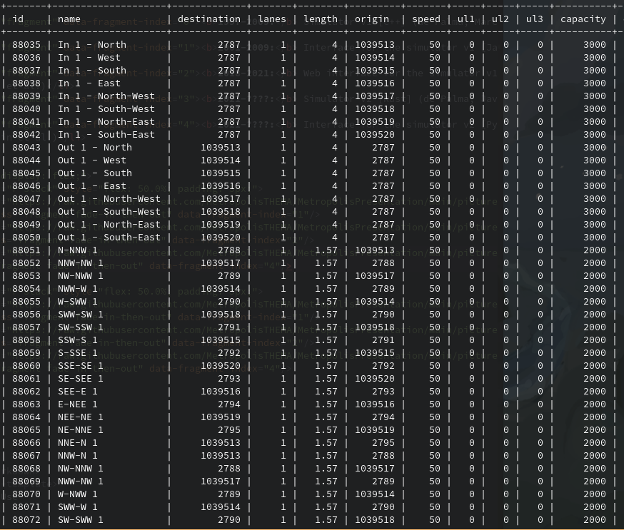
METROPOLIS2 Input Files
- Parameters (JSON)
-
Supply side:
- Road network (Parquet or CSV)
- Vehicle types (Parquet or CSV)
-
Demand side:
- Agents (Parquet or CSV)
- Travel alternatives (Parquet or CSV)
- Trips (Parquet or CSV)
- Optional road-network conditions (Parquet or CSV)
METROPOLIS2 Output Files
- HTML summary
- Aggregated results by iteration
-
Supply side:
- Link-level time-dependent travel times (simulated, expected for last iteration and expected for next iteration)
- OD-level time-dependent travel times (expected for last iteration)
-
Demand side:
- Agent-level results
- Trip-level results
- Routes taken
Units
For consistency and to prevent mistakes, METROPOLIS2 uses the same units for all input and output variables.
| Type | Unit | Example |
|---|---|---|
| Time of day | Seconds after midnight | 8 * 3600 = 28800 is 8 a.m. |
| Time duration | Seconds | 300 (5 minutes) |
| Length | Meters | |
| Speed | Meters / Second | 50 / 3.6 = 13.89 m/s is 50 km/h |
| Passenger Car Equivalent (PCE) | N/A | Usually normalized to 1 for car |
| Flow | PCE / Second | 0.5 PCE/s = 1800 PCE per hour |
| Utility | No specific unit (can be monetary units) | |
| Value of Time | Utility / Second | 15 / 3600 = 0.004167 is 15 $/h |
Mistakes are still possibles, be careful!
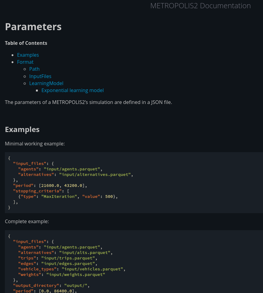
Documentation
The documentation (WIP) is the best way to understand the input and output formats
https://docs.metropolis.lucasjavaudin.comReporting Issues
- Despite all our efforts, various issues can arise when using METROPOLIS2: e.g., errors when running the simulator or Python scripts, simulator panics, unclear documentation
- All issues are collected to a centralized place so that users can learn from each other
- If you face any problem, you should open an issue on this centralized place
- The issue tracker is hosted on Github: https://github.com/Metropolis2/MetropolisExamples/issues
Session 1 Task
- Download METROPOLIS2 on the website and check that it runs correctly on your computer by running the example simulation (See First Run slide)
-
Go through the reference working paper:
Javaudin, L., & de Palma, A. (2024). METROPOLIS2: Bridging Theory and Simulation in Agent-Based Transport Modeling. THEMA, CY Cergy Paris Université.
- Go back to the slides of this session so that you have a global understanding of METROPOLIS2